How to Use an Excel Spreadsheet to Manage Your Tasks

Upgrade your manual to-do list with Traci Williams’ top tips on using Excel to manage your tasks

I am most definitely a LIST person, and love nothing better than creating a nice, tidy to-do list and then getting satisfaction from ticking tasks off the list as I complete them.

However, what tends to happen is that the list grows far quicker than I can tick tasks off it, or priorities change, meaning the task at the top has to be replaced with something more urgent.

As you can imagine, my beautiful, neat and tidy to-do list quickly becomes a complete mess and becomes hard work to maintain.

So, a few years ago I created an Excel version of a to-do list, which I can now update quickly and easily, giving me peace of mind that I won’t forget anything, and I am able to review (and amend) my workload weeks in advance. It also makes it clear when I have any spare resource, which makes planning future tasks easier and saves me from over-committing myself.

This spreadsheet is so useful to me, so I wanted to share it.

It’s a very simple spreadsheet and uses the following functions:

Formula: Weekday / Weeknum / Today / Vlookup
Named Ranges
Pivot Tables
Slicers

In isolation, all simple formulas and functions, but very powerful when used together.

The process to build the spreadsheet is as follows:

1. Create a Task Sheet

I started with a blank sheet, named the sheet ‘Data’, and created columns for relevant data I’d need to enter (you can have as many columns as you need, and don’t have to name them the same as mine):

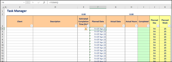
I also formatted the sheet to make it look appealing and applied Filters to the columns to make it easy to navigate.

I will use this sheet to enter each of my tasks on a row.

In column F, I will enter the date I intend to work on the task, and in column G, I will enter the number of hours I expect the task to take.

Top Tip

I keep the time for each task to either a complete hour or 0.5 for a half hour (i.e., don’t complicate things by drilling into individual minutes).

I also never enter more hours in one row than a whole working day, so I usually keep mine to a max of 8 hours. If a task will take longer than this, I’ll enter it into separate rows so I can enter the relevant dates that I intend to work on it into each row.

The columns for ‘Actual Date’ and ‘Actual Hours’ are really just for reference if you wanted to refer back to them to help you with planning, as you can see if tasks take as long as planned. You can leave them blank (or not include them, if they’re not necessary).

The column ‘Completed’ is important, as you can use this as a filter to only view outstanding tasks. It is also important to use the Pivot Table to show only outstanding tasks too.

Enter Formula

There are a handful of formulas I’ve used as follows:

Column F

I’ve entered the =TODAY() formula into this column so that the blank rows contain the current day’s date. (This is just as a helper for when we create the Pivot Table so that there are no ‘blank’ days.)

Column J

This calculates the day of the week that the ‘Planned Date’ falls on (again, to help with the Pivot Table).

This formula works in two parts as follows:

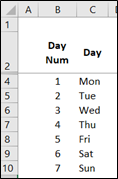
=VLOOKUP(WEEKDAY(F4,2),Day,2,FALSE)

WEEKDAY(F4,2) calculates the day number that the date represents, using the return type ‘2’, meaning that Monday = 1 and Sunday = 7.

The VLOOKUP part is to find the 3-letter abbreviation for the day number. ‘Day’ is a Named Range I have created linked to this data:

Column K

This calculates the week number that the ‘Planned Date’ falls on (again, to help with the Pivot Table):

=WEEKNUM(F4,2)

This formula calculates the week number that the date falls on based on a calendar year, using (as above) the return type ‘2’, meaning that Monday = 1 and Sunday = 7, so it knows when a new week number starts.

All of these columns can be used to apply Filters to the sheet to look for a specific week, weekday or date. Of course, you can also Filter (or use Find) to search for a specific client too.

Named Range

Before I create the Pivot Table, I ALWAYS create a Named Range for the data, and then I use this as the basis of my Pivot Table.

To do this:

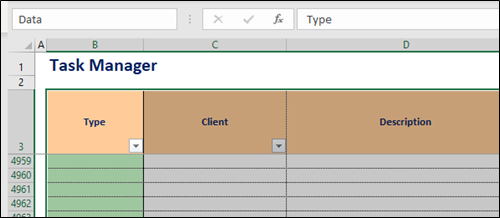
Highlight all of the data, starting from the header row (i.e., C3:K5000)
In the Name box, enter the name for the range and press enter (remember not to use any characters (except _ ) in the name or start it with a number):

Pivot Table

Create a Pivot Table (Insert, Pivot Table):

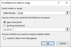
Ensure the Named Range appears in the ‘Table/Range’ box (press F3 for a list of Named Ranges), as opposed to the physical cell reference.

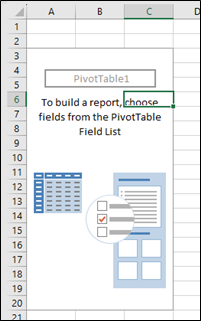
Select ‘New Worksheet’ for where the Pivot Table should be placed, then press OK. A new sheet should appear with the empty Pivot Table on the left-hand side of the page, and the Pivot Table field list on the right:

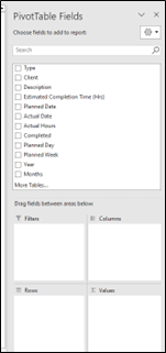
The Pivot Table fields at the top of the Pivot Table field list can be dragged and dropped into the four boxes at the bottom, and the Report on the left will automatically update with relevant information.

I would recommend using the following options in the Pivot Table field list:

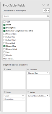
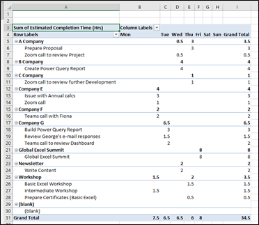
The Pivot Table report would then appear as follows:

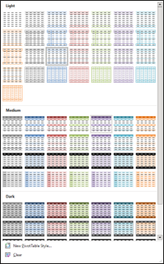
We can then apply different designs to the Pivot Table to make it easier to read. If you click onto the Pivot Table, you’ll notice two extra toolbars at the end of the list at the top of the screen (Pivot Table Analyze & Design).

Select ‘Design’ and select from the many Pivot Table Styles:

Adjusting the Pivot Table

I would also recommend making the following adjustments to the Pivot Table:

Format the numbers in the Pivot Table: Left-click the field in the ‘Values’ box of the Pivot Table field list and select ‘Value Field Settings’. Here you can select ‘Number Format’ to ensure that all numbers will have the same number of decimals.
Change columns widths: Select entire columns on the sheet, right-click, select ‘Column width’, enter desired width.
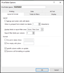
You will also need to stop the Pivot Table automatically adjusting the column widths: Right-click on Pivot Table, choose Pivot Table Options; in Layout & Format tab, uncheck the box ‘Autofit column widths on update’.

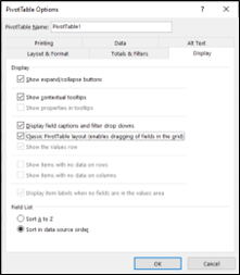
Split Client & Descriptions into separate columns: Right-click on Pivot Table, choose Pivot Table Options; in Display tab, check the box ‘Classic Pivot Table layout’:

Remove Subtotals: In Design toolbar (at top), select ‘Subtotals’, then ‘Do not show subtotals’:

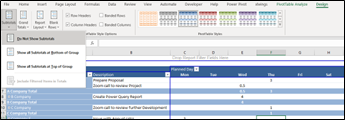
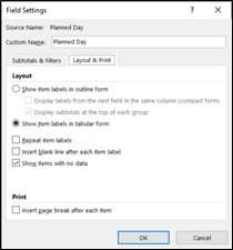
Set Columns to always appear: Left click on field in ‘Columns’ box, select ‘Field Settings’; in Layout & Print tab, check box ‘Show items with no data’:

Now all columns will remain even if there is no data for them.

The report now looks like this:

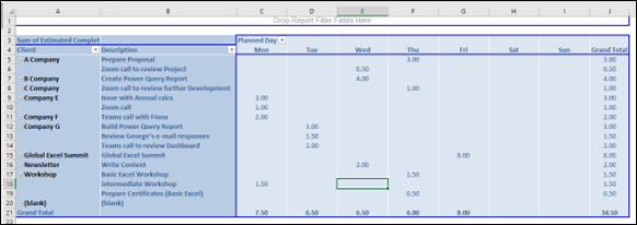
At any time, you can right-click on the sheet and choose ‘Refresh’, and any changes from the raw data will be updated in the above table.

Slicers

The above Pivot Table is looking great; however, it is currently showing ALL of the tasks from the datasheet, and we need to be able to narrow this down to a specific week, and also exclude any tasks that are completed.

We are going to do this with Slicers, which are genius little tools to help us make selections (and they’re easier to use than Filters).

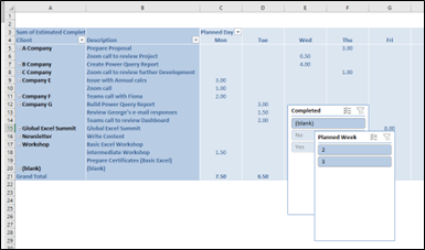
Click anywhere on the Pivot Table, go to the ‘PivotTable Analyze’ toolbar, select ‘Insert Slicer’. A list of all fields will appear; select any that are relevant. I would choose ‘Planned Week’ & ‘Completed’, and they will appear as follows:

Click on each Slicer individually to move and re-size them as required. As you select a Slicer, you will notice a new toolbar at the top (called ‘Slicer’), and this can be used to format them by changing colours, sizes, number of columns, etc.

The Slicer can be used to select a ‘Planned Week’ number, and the data will appear for ONLY the selected week:

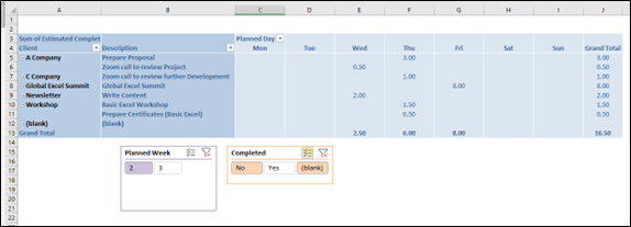
I’ve also made the ‘Completed’ Slicer NOT include anything marked as ‘Yes’; therefore, ONLY the outstanding tasks are being displayed.

Of course, if I want to review the tasks that HAD been completed, I can simply toggle that Slicer too.

All I now need to do is continue entering new tasks into the datasheets, amend the dates of existing tasks, or mark them as complete. Then, when I refresh this Pivot Table, all the information from the datasheet will appear here.

Although this example uses work tasks, this can also be used for personal tasks too, or a mixture of both.

If you don’t have the time to make your own file but would like to try the concept, you can purchase the template from my website: https://www.excelace.co.uk/product/ace-task-manager/

There is also a video demo of this completed file at the above link.