Traci Williams explains the similarities and differences between Vlookup and Index / Match
A lot of people know the Vlookup formula, with varying levels of understanding. Most people learn the Vlookup formula from a colleague and are simply told to ‘put this, there’ with very little explanation as to the purpose or meaning. This is the main reason that people also find the Vlookup formula scary!
Here are some pointers as to how Vlookup works:
Vlookup Purpose
The Vlookup formula matches information between two sets of data and returns values from one set to the other.
The Scenario
We have been asked to prepare a breakdown of the sales data showing the customer, country and salesperson.
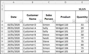
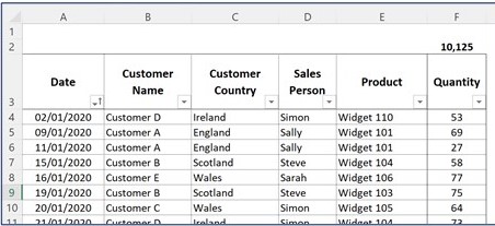
Our Sales Data spreadsheet includes the Date of Sale, Customer, Sales Person, Product and Quantity only:
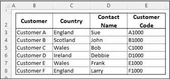
Our Customer Data spreadsheet shows the Customer, Country, Customer Contact Name and Customer Code only.
We need to copy the country information into the Sales Data sheet, from the Customer Data Sheet. This is the perfect time to use the Vlookup formula. We can match information between the two sheets and enter some of it into the Sales Data sheet.
For the Vlookup formula to work, both sets of data must have at least one element of data that will match, and in this instance, it will be the Customer Name. The data must be identical in both sets of data; if there are any typos or mismatching abbreviations, then the formula will NOT work.
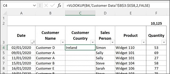
Insert a column for the Customer Country into the Sales Data Sheet and create the formula.
I would recommend using the ‘Formula Wizard’ to enter the formula (i.e., Formula Ribbon, Insert Function, search for Vlookup).
This formula is broken down as:
=VLOOKUP(B4,’Customer Data’!$B$3:$E$8,2,FALSE)
where
B4 – is the Customer Name to search for (and will be matched identically in both sets of data).
‘Customer Data’!$B$3:$E$8 – is the range to search for the Customer in, and as it is on a different sheet, it includes the sheet name and the range of cells.
Note: The first column in the range MUST contain the value to be matched.I’d also usually recommend using a Named Range here instead of the absolute cell references, but this is not essential.
2 – is the column number to be returned when a match is found.
In this instance, this will be the second column. The first column would be Column B, and therefore the second column would be Column C.It is not possible to return a column that is positioned to the left of Column A.
FALSE –is used to return a result if an exact match can be found, whereas using TRUE would return the nearest match. The codes 1 (FALSE) or 0 (TRUE) can also be used instead, as preferred. I tend to use FALSE if searching for text or specific codes, and TRUE if working with date / age or number ranges.
The formula in the above screenshot can simply be copied down the entire column and will return the relevant result for each Customer:
Vlookup Review
The Vlookup formula is brilliant, but it does have its limitations, as you can only return a value that appears in a column after the matched column and you only have two options: TRUE or FALSE (i.e., exact or nearest match).
It only finds the relevant row; the user then must tell it which column to use.
Most experienced Vlookup users are so used to working around these issues that they forget they even exist. However, it’s useful to be aware of, as the next formula will show you how to eradicate them. This formula is a combination of ‘Index / Match.’
Index / Match Purpose
The ‘Index’ formula will look at a range and return a result from the row and column that you specify.
Unfortunately, most of the time we won’t know which row and column we want to use; that’s where the ‘Match’ formula comes in, as we can use that to define the row and column.
Index / Match Method
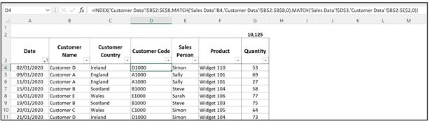
This is the formula that has been used in this example to find the Customer Code:
This formula is broken down as:
=INDEX(‘Customer Data’!$B$2:$E$8,MATCH(‘Sales Data’!B4,’Customer Data’!$B$2:$B$8,0),MATCH(‘Sales Data’!$D$3,’Customer Data’!$B$2:$E$2,0))
This will return the correct Customer Code from the Customer Data.
This looks like a big scary formula, and would put most people off using it, so let me break it down for you:
=INDEX(‘Customer Data’!$B$2:$E$8 – this is the ‘Index’ part of the formula and is saying to look in the range B2:E8 on the Customer Data sheet.

MATCH(‘Sales Data’!B4,’Customer Data’!$B$2:$B$8,0) – this is the first ‘Match’ and will return the row number to use.
This formula is saying to match the value from B4 within the range of B2:B8 on the Customer Data sheet and find an exact match (this is what the 0 at the end represents).
MATCH(‘Sales Data’!$D$3,’Customer Data’!$B$2:$E$2,0)) – this is the second ‘Match’ and will return the column number to use.
This formula is saying to match the value from D3 within the range of B2:E2 on the Customer Data sheet and find an exact match (this is what the 0 at the end represents).
The formula would return the result for the matches first, which would make the formula look like this:
=INDEX(‘Customer Data’!$B$2:$E$8,5,4) – this is saying: from the range B2:E8 on the Customer Data sheet, what is the value in Row 5, Column 4?
Index / Match Review
So, as you can see, the Index / Match formula can return a result from any column, not just columns to the right of the match. It can also return both row and column (unlike Vlookup). The Match formula also gives 3 options: Less Than (1), Exact Match (0) & Greater Than (-1), so it gives greater flexibility than Vlookup.
The Index/Match is a little trickier to use than Vlookup, but it is real genius, and I’d really recommend trying to understand it a little better.