Traci Williams explains how to set up a spreadsheet so that you can track your time
I used to get really upset with myself for never seeming to get to the end of my to-do list each week.
Every week, I thought I’d been careful with working out how long tasks would take and making sure I had enough time to get them all done, but every Friday evening, I’d be left with incomplete tasks, and I’d have to work over the weekend to catch up.
I decided to keep track of what I did with my time so I could hopefully find out where I was going wrong. It goes without saying that I used a spreadsheet to help me.
It’s a very simple spreadsheet and uses the following functions:
- Named Ranges
- Data Validation
- Countif
In isolation, all simple functions, but very powerful when all three are used together.
The process of building the spreadsheet is as follows:
1. Create a List of Categories
I started by making a simple list of the categories of time I wanted to track, on a sheet named ‘Lookup’:
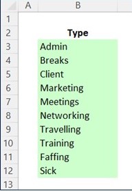
As you can see, this list is on the range B3:B12, so if I wanted to refer to this list on another sheet, the cell reference would need to also include the sheet name AND dollar symbols to freeze the cell references, so it would look like this:
=’Lookup’!$B$3:$B$12
All those dollar symbols can make it difficult to read, especially if you’re using Column ‘S’ and/or Row ‘5’ too. So, I always prefer to give that range of cells a name so I can refer to that name instead of the cell references.
Named range
The simplest (and quickest) way to create the named range is to highlight the entire range including the heading (e.g., B2:B12). Then go to the Formulas ribbon and select ‘Create from Selection’:
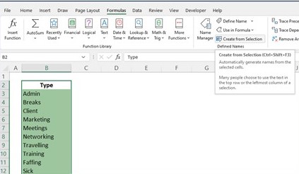
This screen will appear; select ‘Top row’ and press OK.
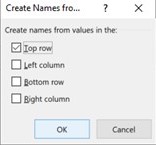
The top row will be used for the name of the range but will not be included within the range. This is what we need, as that is just the heading, not one of the categories.
You can use the ‘Name Manager’ from the ‘Formulas’ ribbon (above) to edit or amend (or delete) any of the named ranges after they are created.
Note
I colour code everything, so the cells above are green, as this reminds me that these are the cells included in my named range.
2. Create a Daily Sheet
I started with another blank sheet, naming the sheet ‘Monday’, and typed Monday’s date into cell B1. I then formatted the date so it would include the day of the week as well as the date, month & year.
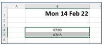
In cell B4, I entered the start time for the working day as 07:00 – not that I start every day at 7 a.m., but I could if I needed to.
I decided I wanted to analyse how I spent my time in 15-minute intervals, so in the row below, I entered the time 15 minutes later (i.e., 07:15). You could make this 30-minute intervals by entering the time as 07:30.
Note
Times in Excel are expressed with the colon ( : ) separator.
To repeat these intervals for the duration of the day, highlight the two cells together; you will see a tiny square at the bottom right of the selection:
Hover the mouse over this square until it turns into a black cross, then hold down the left mouse button, keep it pressed and drag the cells down the sheet until approx. row 70 (if in 15-min intervals). This will repeat the sequence of intervals down the sheet until approx. 23:45.
Include headings at the tops of the columns, and format the cells to make it easier to read:
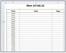
Column D (Type) is where we want to enter the relevant category so that we can analyse the type of time used. I am prone to typos (no matter how careful I try to be), so I would include ‘Data Validation’ in this column, which means I can restrict what can be entered into the cells. In this instance, it would be a ‘pick list’ to prevent typos.
Data validation
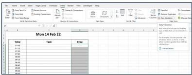
To start, highlight all the cells where you want to include the pick list, then go to the ‘Data’ ribbon and select ‘Data Validation’:
This screen will then appear:
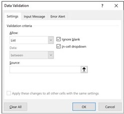
In the ‘Allow’ box, I have selected ‘List’, which is how we can create the pick list.
In the ‘Source’ box, we need to tell it where the list is, and this is where we would usually see the cell reference mentioned above (=’Lookup’!$B$3:$B$12). However, as we have a named range, we can use that now. AND there is a lovely keyboard shortcut we can use to find it, too.
Make sure the cursor is flashing in the ‘Source’ box, then press the F3 key on the keyboard and the list below will appear:
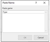
Select the relevant named range and press OK. This will go back to the screen above, and you should press OK again to complete the data validation.
You will then see (on every cell that was selected) an arrow appear to the right of the cell, which contains the pick list from our list of categories on the ‘Lookup’ sheet.
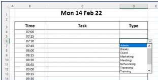
Now you can simply select from that list in order to populate the cell. This makes it quicker to enter and prevents typos or different categories being used.
This sheet can now be used to enter the tasks completed every 15 minutes of the day and allocate them to a category.
3. Create Summary Table Using Formula
We now need to include some formulas to summarise the information.
The summary table needs to have a row for each category, and they should be linked to the ‘Lookup’ sheet.
In cell G4, begin entering a formula by pressing the = key, then simply navigate to the Lookup sheet, select cell B3 and press enter.
This will include the value from cell B3 (on the Lookup sheet) on the ‘Monday’ sheet. If the value on the ‘Lookup’ sheet should change, so, too, will the value on the ‘Monday’ sheet.
This formula can be copied down to row 13 and it will automatically update the row numbers as it moves down.
In column H we will include a formula to calculate the total minutes for each category, and that will be a ‘Countif’ formula. Before you enter the formula, I recommend selecting some categories in column D, just so there is some data to check if it is working.
Select cell H4 and enter the formula:
=COUNTIF($D$4:$D$71,G4)*15
This formula is saying:
Count how many items are in the range of D4:D71, where the value is equal to cell G4, then multiply the answer by 15 (as I’m using 15-minute intervals).
On row 4, this means: Count how many times ‘Admin’ appears in column D, then multiply it by 15 mins.
Note
The cell reference $D$4:$D$71 includes dollar symbols. This is so that it stays the same when the formula is copied down into the other rows. Conversely, the cell reference G4 does NOT contain any dollar symbols, so the row number WILL update as this formula is copied down into the other rows.
This formula can now be copied down into the rows to row 13, and include a sum total at the bottom:
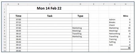
These numbers now show the total time spent on each activity and can be compared to what the planned time was supposed to be.
You could then format the sheet to make it more appealing and copy the sheet, so you have one for each day of the week.
For me, this file was invaluable as I completed it honestly and accurately for a couple of weeks. On reviewing the results, I realised I was spending approx. 40% of my week on tasks such as travelling / admin and (over-running) meetings. This helped me to plan my time more realistically to include time for these things.
Also, inadvertently, I realised I became more productive, as I knew that every chunk of time was being monitored, and therefore, I tried to make sure I was always doing something productive.
If you don’t have the time to make your own file but would like to try the concept, you can download the FREE template from my website:
https://www.excelace.co.uk/standard-products/ace-time-tracker/