It is imperative that we check, identify, and resolve spreadsheet errors efficiently so that the data can be relied on, explains Traci Williams
One of the biggest concerns about spreadsheets is the worry about getting things wrong and making mistakes.
I researched how common it is to find errors in spreadsheets, and found these (quite alarming) statistics*:
High Error Rates: Studies suggest that up to 88% of spreadsheets contain errors. This figure varies depending on the complexity of the spreadsheet and the user’s expertise.
(Source: Panko, 1998; Raymond R. Panko, Spreadsheet Errors Research)
Human Error: About 40% of errors in spreadsheets are caused by simple human mistakes such as typos, incorrect formulas, or improper cell referencing.
Error Detection: People tend to detect only about 50% of errors in their spreadsheets during a manual review.
*ChatGPT-4o
Errors can be caused in many ways, such as incorrect data entry, mistakes in formulas, and broken (or incorrect) links or ranges. And any one mistake can also carry forward into subsequent worksheets or workbooks too.
Spreadsheet errors can be as simple as causing ‘re-work’ but can also lead to poor decisions being made with severe financial implications. So, we must know how to identify (and resolve) any errors to trust and rely on spreadsheets.
Understanding Errors in Excel
Excel is always trying to help us, so even the error message you see will be trying to convey the cause of the error, as follows:
- #DIV/0!: Division by zero or empty cells
- #N/A: Value not available, often seen in lookup formulas
- #VALUE!: Incorrect data type (e.g. cells contain text and not values)
- #REF!: Invalid cell reference, often due to deleted cells or ranges
- #NAME?: Misspelled function names or unrecognized names
- #NUM!: Invalid numeric operations (e.g., square root of a negative number)
- #NULL!: Incorrect use of range operators
Built-in Error Checking Tools
Excel has some functions we can use to identify or prevent errors, such as:
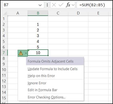
Error Indicator (green triangle):
A green triangle will appear in the top left corner of a cell as a warning. Clicking on the exclamation mark will show the message and some suggestions for resolution:
Formula Auditing toolbar
This appears in the ‘Formulas’ ribbon:
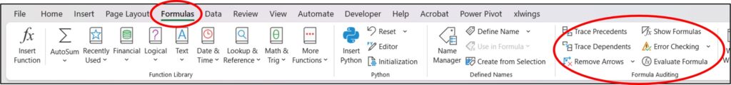
Trace Precedents
Identify cells feeding into the formula.
Trace Dependents
See which cells depend on the current cell.
Evaluate Formula
Step through a formula to debug issues (this is my favourite!).
Error Checking Dialog Box
Review errors across the sheet.
Data Validation
This function enables you to restrict the values that can be entered into a cell, preventing incorrect information from being entered at all. Input and error messages can also be defined to provide guidance and clarity if an error occurs.
This can be found on the ‘Data’ ribbon and is one of my favourite functions in Excel, as it prevents me from entering typos and incorrect dates (which I do A LOT!).
Circular reference checker
Circular reference alerts will appear automatically when a formula refers to itself, directly or indirectly.
In the example below, the formula in cell B7 also includes the cell B7:
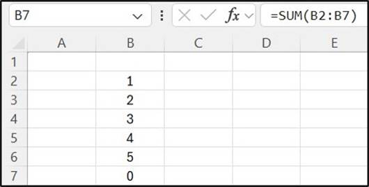
When this formula is entered, the error message below is displayed:
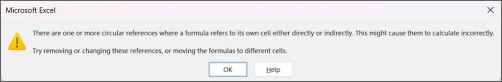
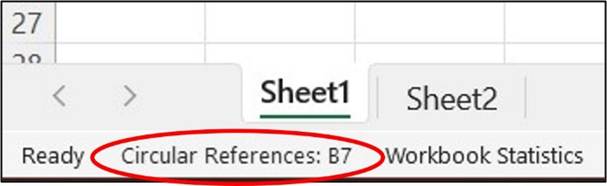
Also, on the bottom left of the screen, this warning will appear, indicating the specific cell where the circular reference can be found:
There is no specific guidance for resolving a circular reference, but reviewing the formula in the specified cell should be enough to find and resolve the issue.
Note
If you are on the sheet which contains the circular reference, the note above will include the cell reference. If you are on a different sheet, this will just say ‘Circular References’ with no indication of the cell reference.
Error Handling within Formulas
Using error-handling functions
Sometimes, we will have errors, as we simply haven’t input all of the data yet, or in some cases, it may not be relevant. When the error messages are visible, it can look untidy and like something has broken, but errors will also prevent Sum / Subtotal formulas from calculating using the rest of the range.
In these circumstances, we can anticipate errors and include within the formula how to handle these, as follows:
IFERROR
Anticipate errors and replace with a specific value.
Example: =IFERROR(A1/B1, 0)
This formula divides A1 by B1, but if there is an error, will return 0 (instead of #N/A).
IFNA
Specifically handles #N/A errors.
Example: =IFNA(VLOOKUP(“Item”, A2:B10, 2, FALSE), “Not Found”)
This formula will lookup ‘Item’ within the range A2:B10 and return the item in that row, from column 2, but if there is an error, will return the text ‘Not Found’ (instead of #N/A).
Preventing errors in formulas
Use ISNUMBER, ISBLANK, ISTEXT, etc. to validate inputs before a calculation is made.
Example: =IF(ISNUMBER(A1), A1*2, “Invalid Input”)
This formula will check if A1 is a number; if it is, it will calculate A1*2, but if not, it will return the text ‘Invalid Input‘ (instead of #VALUE!).
Logical conditions to avoid errors
Use IF, IFS, COUNTIFS, etc to check conditions are met before a calculation is made.
Example: =IF(B1=0, “N/A”, A1/B1)
This formula will check if B1 equals 0; if it does, it will return 0, but if not, it will calculate A1/B1 (instead of #DIV/0!).
Custom Techniques for Error Checking
Using conditional formatting
Include conditional formatting using a formula such as: =ISERROR(A1).
This will highlight cells containing errors.
This function can also be used to highlight blanks, duplicates, or inconsistent data formats.
Error checking with functions
LEN for text consistency, especially in ID fields where you need a specific number of characters.
TEXT functions for standardizing data formats; this is really useful for codes that may look like numbers and ensures consistency.
Named Ranges and Table References
Using a Named Range or Table References reduces the chance of errors, as fixed and consistent references will be used as opposed to individually selecting cells or ranges each time they are used. I love to use Named Ranges when sorting data, as I know that the correct range has been selected (plus, it’s quicker than manually selecting).
Also, when using Named Ranges in formulas, it makes them look neater, they make more sense (providing you use a relevant name for the range) and they will automatically update as the Named Range changes, meaning you won’t need to update individual formulas.
Error Prevention Strategies
Of course, preventing errors from occurring is far preferable to correcting them afterwards, and there are a few options for this:
Data Validation
As discussed above, using Data Validation to include dropdown lists or specify data formats can prevent errors from occurring at all.
Template design best practices
If you are creating a template to work from, use clear naming conventions for ranges and worksheets for simple identification and ease of use.
Keep variables separate from raw data so they are easily accessible to refer to or amend. Have formulas refer to the variables to prevent formulas from needing to be amended.
Documentation and training
Add comments or notes to explain complex formulas or data input requirements.
Use a consistent colour-coding scheme for input, output, and calculated cells, as this is visually more appealing but also clearer to discuss (e.g., “Yellow cells contain formulas” is far simpler than “Cells B2:D40 & B1:E1 contain formulas”).
Understanding how a user is using a spreadsheet can highlight a training need. I see a lot of users use ‘cut & paste’, and this tends to break any dependent formulas. I simply educate them to use ‘copy & paste’, then delete the original entry to prevent this.
Regular Audits & Control Checks
Always complete random checks on some of the data to ensure that it logically makes sense and there are no inconsistencies, as even given all the control checks, the user could still manually enter incorrect data.
Also, include some simple control checks to confirm totals are reconciled such as =D10=A10 This will return a TRUE or FALSE result if the two cells match. Of course, you could also use a simple =D10-A10, which will return the difference between the two cells.
Conclusion
Errors in spreadsheets can be caused very easily and can have disastrous consequences, so it is imperative to be able to check, identify, and resolve errors efficiently in order to be able to rely on spreadsheets.
An even better approach is to build spreadsheets that reduce (or eliminate) the likelihood of errors being made at all by employing some of the techniques discussed above, and use these as best practices always.
As errors are detected, don’t just correct them, but try to adapt the spreadsheet to ensure that error cannot re-occur.