Traci Williams explains how to use Excel’s functions and features to create a budget for your project
Managing a budget is essential in lots of situations, both in your personal life (e.g., household budget) and also in your working life (e.g., projects). Being able to keep within your budget limits takes careful planning and organisation and can be the difference between success and failure.
Excel is an amazing tool to help with budgeting, as it has lots of powerful functions and features to help calculate data and highlight trends or issues.
This article delves into how to best use some of Excel’s features to your benefit when working with budgets for a project.
Setting Up Your Budget Template
When setting up your spreadsheet, I always advise you to ‘keep it simple’ and keep the end goal in sight.
Consider the following:
Structure
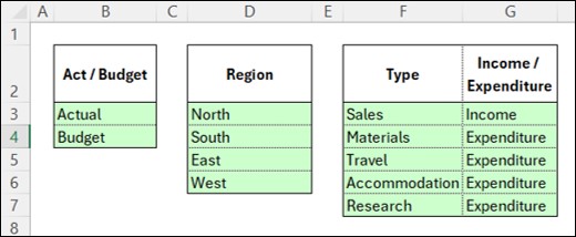
Define categories (e.g., Income & Expense / Actual & Budget / Department / Product / Person / Region, etc.) that are relevant to your project.
I’d recommend having a separate sheet for these categories, with each linked to a ‘Named Range’ so they can easily be used within ‘Data Validation’ (pick lists) or formulas:
This structure would also define the column headers for your data collection:
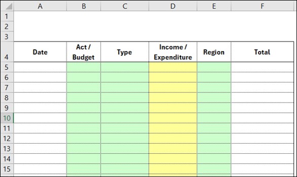
Formatting
Use cell formatting for easy identification of data (and input type). In the above example, green indicates a pick list (linked to Set Up lists (above)), whereas yellow indicates formulas and therefore no manual entry required.
Formulas
Include formulas to populate your data automatically (where applicable) to minimise the amount of manual work (e.g., use a Vlookup formula linked to the ‘Type’ field). This reduces the amount of manual work, making the process quicker, and also increases accuracy.
*Of course, these examples are just suggestions; you can have as many (or as few) columns of data as necessary.
Data entry
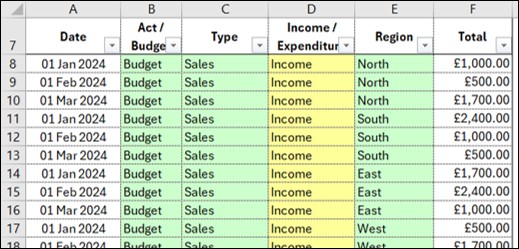
Now you have your structure, formatting and formulas ready to go, you will need to enter the budget and actuals (as they happen).
Use a row for each detail (e.g., Date, Act/Budget, Region, Type and Total Value, as per this example):
Of course, this layout does not appear to be ‘pretty,’ nor does it summarise any of the information, so the temptation would be to collect the information AND summarise it at the same time.
However, this temptation is to be avoided, and you will thank yourself later!
This layout is perfectly functional, simple to input and easy to update or amend. We can worry about making it ‘pretty’ later.
Keeping the input as simple as possible will make it easier and quicker to put the data together so that you can spend longer on analysing and interpreting the results.
Analysis and interpretation
The data can be analysed using formulas or Pivot Tables (or both) with the ultimate aim being to compare actuals against budget, by region and over time, ensuring there is no overspend.
Simple summary
Here is a simple summary at the top of the sheet, showing totals for act vs budget with a variance:
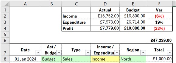
This summary uses simple SUMIFS formulas, as follows:
D2: =SUMIFS($F$8:$F$121,$D$8:$D$121,$C2,$B$8:$B$121,D$1)
$F$8:$F$121 – The range of cells to sum
,$D$8:$D$121,$C2 – The first criteria range & criteria (i.e., match C2 “Income” in column D)
,$B$8:$B$121,D$ – The second criteria range & criteria (i.e., match D1 “Actual” in column B)
Note: The use of dollar symbols ($) on the ranges in this formula means that it can simply be copied into all cells: D2:E3
This is a very simple summary; it does not break the variances down into region, month or expense type.
Detailed summary
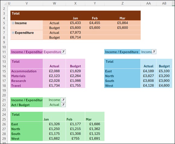
In order to achieve a detailed analysis (by region, month or expense type), I’d recommend using a Pivot Table:
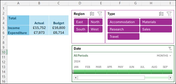
In the above example, the Pivot Table can be seen on the left (blue) and shows a similar summary to that above. However, alongside this Pivot Table are slicers (purple) and a timeline (green), where we can drill into the detail in the Pivot Table by simply making a selection like this:
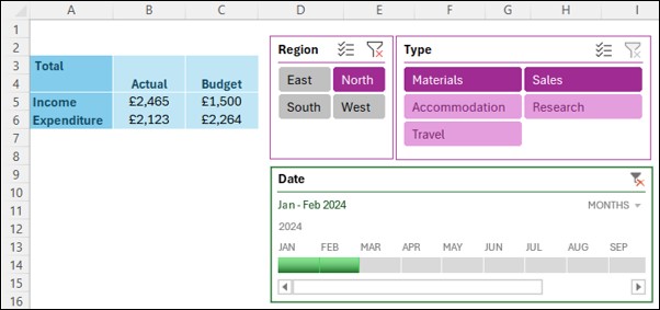
In this instance, the region ‘North’ has been selected from the slicer, and the months Jan-Feb have been selected in the timeline. This shows the Pivot Table has adjusted to show the results for those selections.
The Pivot Table can include variances and profit calculations by use of ‘Calculated Items,’ but they can be difficult and clunky to use. A far easier option would be to simply include manual formulas alongside the Pivot Table (provided the Pivot Table layout will not change, of course).
Visual summary
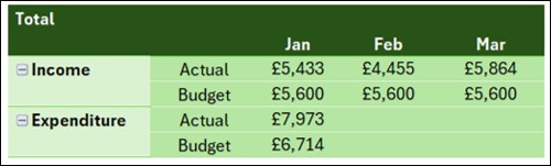
As lovely as Pivot Tables are, they are not always the easiest to read the data from, so we could display the data using a Pivot Chart (linked to the Pivot Table) like this:
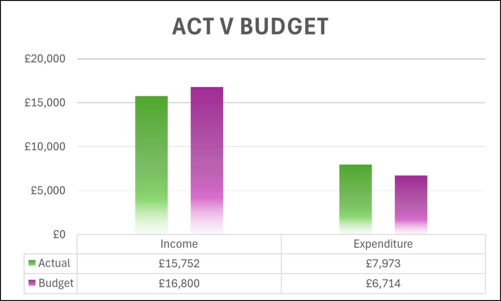
Although this chart does not include the variances, the distinction is perfectly visible to see at a glance, potentially making the calculation of variances unnecessary.
We could even create a chart per region like this so we’re able to compare the regions too:

The absolute beauty of a Pivot Table is that it can be refreshed at the touch of a button if (or when) the data changes, and you can also have multiple Pivot Tables & Charts linked to the same data, showing analysis in many different ways:
Charts tell a story far more easily than a list of numbers and are usually the better choice when trying to communicate the story to others.
Conclusion
It is important to input data in a timely manner in order to be able to take corrective action on any issues it may highlight.
Taking the time to set up a very simple budget structure at the beginning of a project will save you hours of pain every month (or week!) when trying to report on it.
Having this type of analysis can also highlight any data entry / misallocation issues and enables them to be put right very quickly.