In this extract from her new book “Dirty Data: Excel techniques to turn what you get into what you need” Melissa Esquibel explains the importance of a good list in excel
To really open up the tool set in Excel, you must have an optimally structured list. So many of my consulting projects begin with restructuring the list. When you try to address the way you want to see it as a finished report before you address how you want to work with the data to create information, you end up with restrictive choices, choices which don’t allow you to sort or filter properly, perform calculations easily, and use advanced tools, like pivot tables or queries.
Some of my clients have watched in horror as I’ve unmerged cells, deleted rows and columns, and transformed their “print happy” worksheets into reporting tools. It’s like when the plastic surgeon must break your nose to fix it. I promise you this is less painful and less expensive! And, you will breathe easier once it’s done. (Yeah, OK. That was a stretch.)
The optimal list has the following characteristics:
- No merged cells from the column header row down
- One row to one record, no multi-row records
- Descriptive, single cell column headings
- Consistent data types in columns (all dates, all amounts, etc.)
A good test is to click a cell in the middle of your data and press Ctrl+A. Does it select all of your data? Now, turn Filter on, either from the ribbon (Data tab, Sort & Filter Group, Filter button) or using the shortcut Ctrl+Shift+L. Do the drop-down arrows appear at the top of each column as you would expect? If your data passes these two tests, you’re about 90% there. The rest won’t be determined until you do something with the list, like pivot it or create a table. Not working as it should? Check out these tips to repair the damage.
Tip #1 – Multi-row records
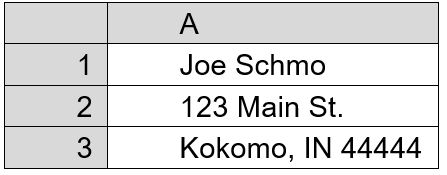
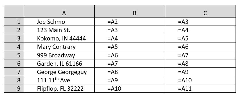
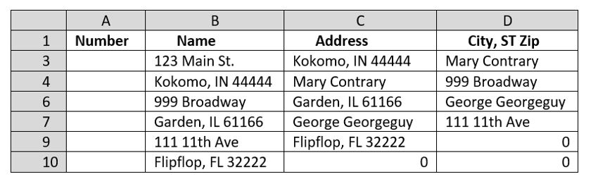
Think of how you might see a mailing label. The name on top of the address on top of the city, state/province and postal code. This can’t be used as is for any type of filtering or sorting on postal/zip code, state/province, or last name.
We have this:
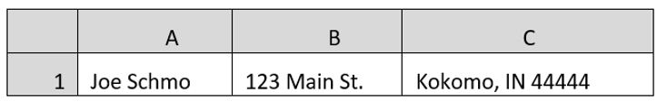
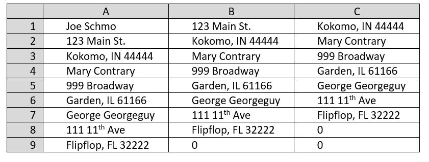
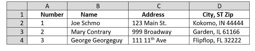
We need this:
If we’re only talking about a few rows of data, we can use the Transpose paste option.
Select the 3 rows of address data and copy (Ctrl+C)
From the Paste button drop-down arrow in the Clipboard group on the Home tab, choose the Transpose option, or just type a T with the drop-down button options showing. (To break apart the name into first and last, and the city, state and zip, into their own columns, see Chapter 4 – Intelligent Strings).
If you have a lot of rows, you could try this more advanced approach using formulas. I’ve extended the example a bit for this technique. This will look crazy, but, I promise, in the end, it works like a charm. For the first row, enter the formulas as shown below.
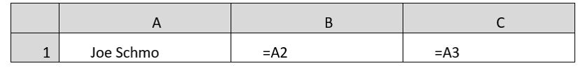
Now, select B1 and C1. You’ll notice a little black box in the lower right corner of C1. That’s the Autofill Handle. Double-click it. That should fill the formulas down.
That yields the following. DON’T PANIC! It’s supposed to look like this.
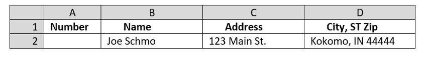
Insert a new column above and to the left of Column A and type headings.
Type a 1 in A2.
Select A2 through A4. And, double click the Autofill Handle.
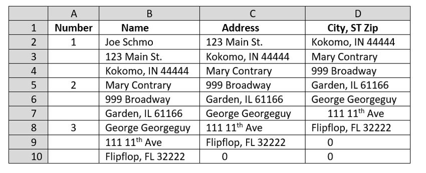
Select Columns C and D by clicking and dragging across both column letters, or select Column C from the letter and using Shift+Right Arrow. Copy them (Ctrl+C).
Then, choose Paste Values. This replaces the formulas in C and D with the actual results.
Now, turn on Filter (Ctrl+Shift+L) and filter Column A to show only those cells with blanks.
That will give you this mess.
Select from the row numbers (very important!) to include all rows of filtered data.
Press Ctrl+- (minus or dash) or right-click and choose Delete Row.
DON’T PANIC! It’s supposed to look like you just deleted all of your data.
Turn filter off (Ctrl+Shift+L) or use the ribbon button.
Voila! Your data is following the one row, one record rule.
Tip #2 – Instead of blank columns
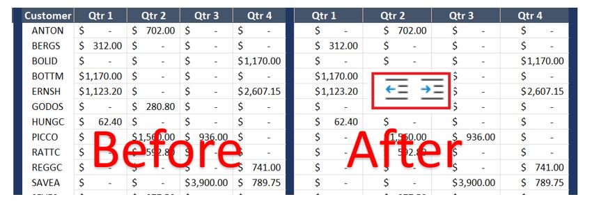
Sometimes, worksheets are easier to read if there is more horizontal separation between columns.
For example, if you have applied the Accounting format ($ flush with the left cell border) and the cell to its left is sized to fit the text, it might seem like just a narrow, little column would make it all better.
Just like replying emotionally to a controversial social media post, it can feel good for a few minutes, but ultimately, there may be a price to pay.
To avoid breaking your list with these “spacer” columns, use the indent feature instead. You get all the benefits of optimal horizontal spacing without the regret when you try to sort, filter, or pivot your data.
Tip #3 – Instead of blank rows
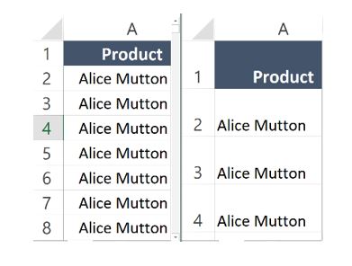
Like our “spacer” columns above, “spacer” rows are also the kiss of death if you want to do things like sort or filter without having to manually select the entire dataset.
Instead, try this trick. Select your rows by clicking on the row number, followed by Ctrl+Shift+Down Arrow. Now, click and drag the bottom border of one row down to make it a bit bigger. Voila! “double spacing” and no broken data.
Tip #4 – Instead of merged cells
So many good intentions for spreadsheets are dashed by merged cells. “Yes, but Merge & Center makes it look so preeeeetty!!!” OK, but what if I told you that you can get the “pretty” without breaking the matrix?
Begin as you normally would by selecting your text and the cells across which you want to center it. Now, click on the dialog box launcher in the Alignment group and change the Horizontal setting to Center Across Selection.
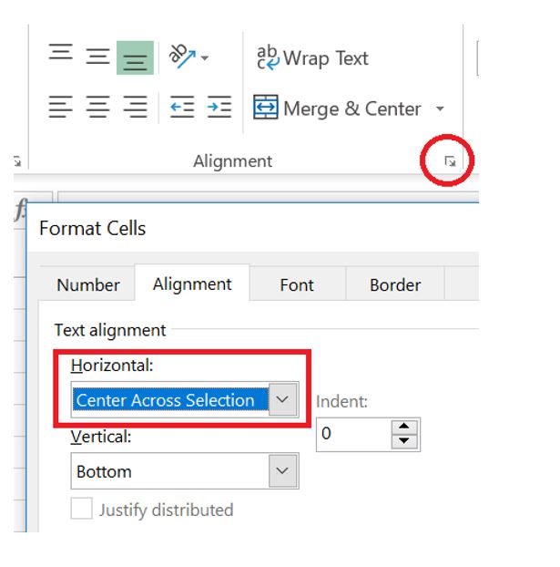
It appears the same after applying this format, but individual cell definitions are preserved.