
In the second part of this series on Dynamic Arrays, Traci Williams introduces more formulas that will make you look like an Excel ACE!
In the last article, we explored Dynamic Arrays (if you haven’t read it yet, go and check it out) such as UNIQUE, SORT, FILTER, and SEQUENCE. These are quite straight forward and simple to follow.
In this article, we are going to look at some more complex Dynamic Arrays, such as HSTACK, VSTACK, TAKE, DROP, CHOOSECOLS, and CHOOSEROWS. They are a little trickier, but just as ACE!
Complex Dynamic Arrays
These formulas let you reshape, extract, and stack data with a single function, giving you SQL-style slicing and shaping capabilities without needing to venture outside of your spreadsheet.
Here’s a quick summary of their purpose:
1. HSTACK / VTSACK
What it does: Combines multiple ranges into one table.
EA Use Case: Merge client lists with contact details from different sheets into one clean view.
2. TAKE
What it does: Returns the first or last n rows / columns from a range.
EA Use Case: Show only the top 10 performers for a report, or the latest entries received.
3. DROP
What it does: Removes a set number of rows / columns from the start or end of a range.
EA Use Case: Strip out header rows or old data before sharing.
4. CHOOSECOLS / CHOOSEROWS
What it does: Extracts only the columns / rows you specify, in the order you want.
EA Use Case: Deliver a simplified version of a dataset containing just the key information a leader wants to see.
5. Combinations
What it does: Combines above functions for even more powerful functionality.
HSTACK – Combine Data Horizontally
What it does:
Joins multiple ranges side-by-side (left to right horizontally). Use it when you want to align datasets that have the same number of rows.
Example
Suppose you have two tables like this:
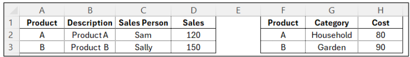
We could use the HSTACK formula to combine data from the two tables, as follows:
Formula
=HSTACK(A1:A3,D1:D3, F1:F3,H1:H3)
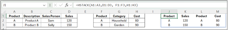
This formula only selects the columns A, D, F, and H.
Note that due to the dynamic nature of this formula, it is simply entered into cell J1 and it ‘spills’ into the relevant cells automatically. No need to copy the formula or freeze the cell references (with $ symbol).
VSTACK – Combine Data Vertically
What it does:
Stacks ranges top-to-bottom. Use it to append lists or combine monthly / regional tables.
Example
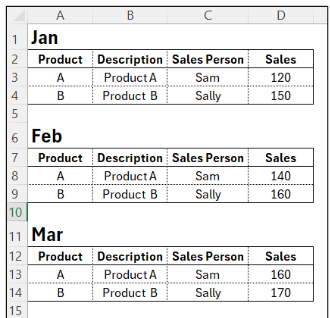
If your data is laid out like this, it is difficult to summarise or work with:
We could use the VSTACK formula to combine this data, as follows:
Formula
=VSTACK(A2:D4,A8:D9,A13:D14)
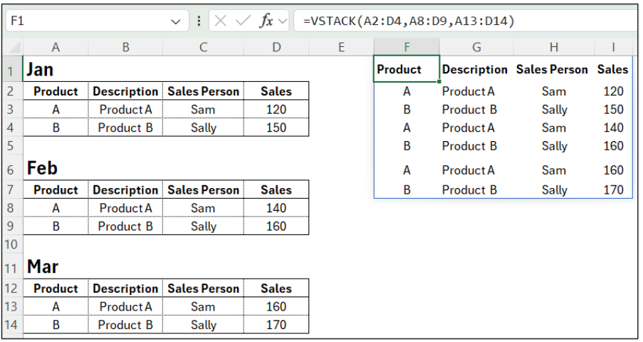
Note: to avoid repeating headers, I included the headers from the first section (row 2) but excluded them from the subsequent ranges.
This formula removes the need to either manually copy and paste or delete rows, and it also eliminates the need to amend the raw data at all, which makes it far more robust. Plus, it’s literally one formula in one cell, so it’s super quick too.
TAKE – Extract a Set Number of Rows or Columns
What it does:
Returns the first or last n rows or columns.
- Positive number >> from top/left
- Negative number >> from bottom/right
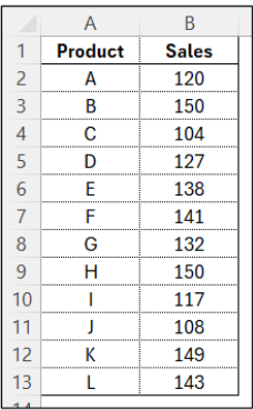
With a dataset like this with multiple rows of sales values, there are several things we can do with the TAKE formula:
Example 1
We can TAKE the first 5 rows of data:
Formula
=TAKE(A2:B13, 5)
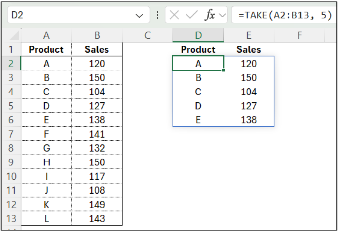
Notice that this formula is in cell D2 and also uses the data range starting from row 2, as I have manually input the headers into row 1.
Of course, we could also have entered the formula into row 1 and used the data range starting from row 1: =TAKE(A1:B13, 6), but we would have had to include 6 rows, as the first row would be the headers. This works perfectly when taking data from the top, but if we take data from the bottom (next example), it doesn’t work.
Example 2
We can TAKE the last 5 rows of data:
Formula
=TAKE(A2:B13, -5)
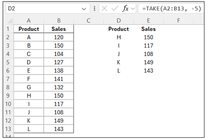
Notice that this formula in cell D2 is identical to that above, except it has a minus sign before the number of rows to TAKE (from the bottom).
Example 3
We can TAKE the last 5 rows AND only the first column of data:
Formula
=TAKE(A2:B13, -5,1)
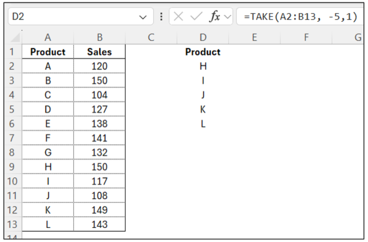
This is useful if you only want a list of the last 5 products (and NOT the sales values).
DROP – Remove Rows or Columns
What it does:
Removes a number of rows or columns from the top/left or bottom/right.
- Positive number >> drop from top/left
- Negative number >> drop from bottom/right
Using the same table as above
Example 1
We can DROP the last 7 rows of data:
Formula
=DROP(A2:B13, -7)
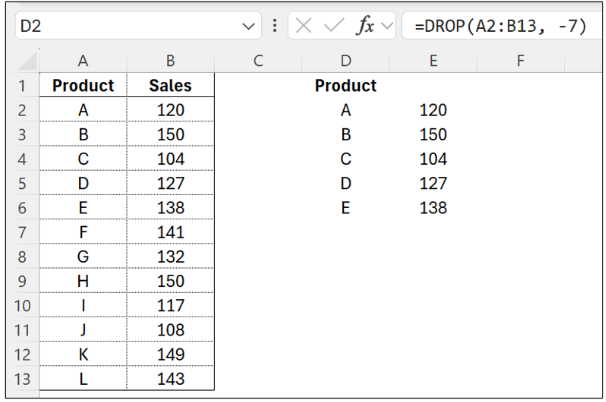
The result shows the top 5 items in the list (and drops the last 7 from the bottom of the list).
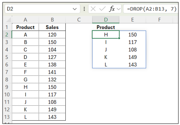
Alternatively, we could drop the first 7 items from the list to display the bottom 5 on the list:
Formula
=DROP(A2:B13, 7)
CHOOSECOLS – Pick Columns by Position
What it does:
Extracts specific columns by index number. If your table has many columns, this function lets you rearrange or reduce it quickly.
Example 1
Return just the Feb and Jan columns (in this order).
Formula
=CHOOSECOLS(A1:D4,3,2)
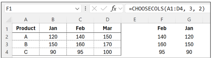
Excel returns the specified columns in the defined order.
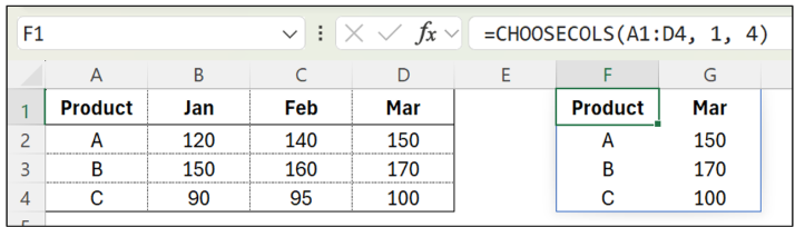
Example 2
Return only the first and last columns.
Formula
=CHOOSECOLS(A1:D4, 1, 4)
Example 3
Use a sequence to dynamically select columns to return.
Formula
=CHOOSECOLS(A1:D4, SEQUENCE(3))
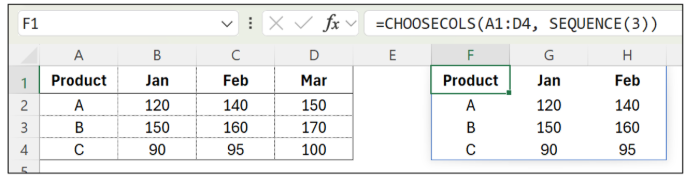
This extracts columns 1, 2, and 3 without needing to specifically list all of the individual columns.
CHOOSEROWS – Pick Rows by Position
What it does:
Returns specific rows based on row numbers. If your table has many rows, this function lets you select specific rows only.
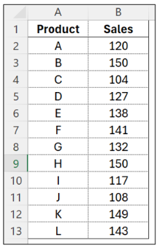
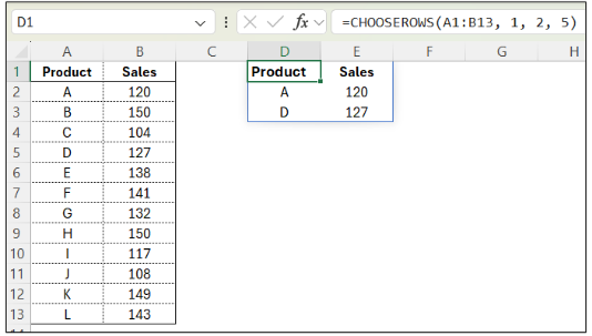
Example 1
Return rows 1, 2, and 5.
Formula
=CHOOSEROWS(A1:B13, 1, 2, 5)
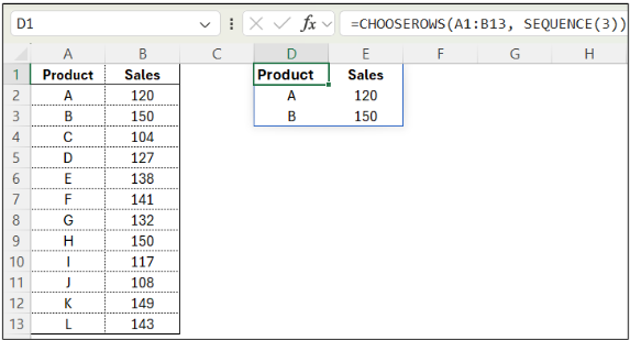
Example 2
Return the first 3 rows using SEQUENCE.
Formula
=CHOOSEROWS(A1:B13, SEQUENCE(3))
Combinations
These functions become even more useful when you start combining them.
Example 1
With data such as this:
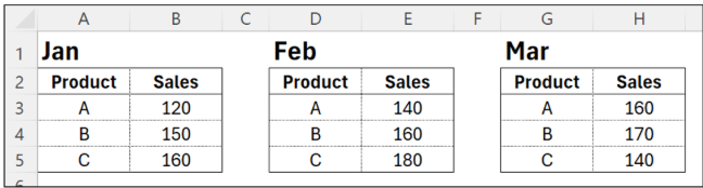
Combine all tables, remove headers, and keep top 7 rows.
Formula
=TAKE(VSTACK(DROP(A1:B5,2), DROP(D1:E5,2), DROP(G1:H5,2)),7)
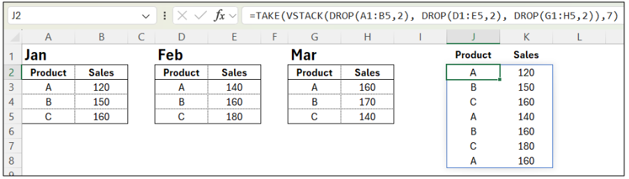
What it does:
- DROP(…,2) removes each table’s header & month.
- VSTACK appends them.
- TAKE(…,7) gives the first 7 rows of the combined dataset.
Example 2
With data similar to that below, we can use a combination of dynamic formulas to build a custom report with selected columns only.
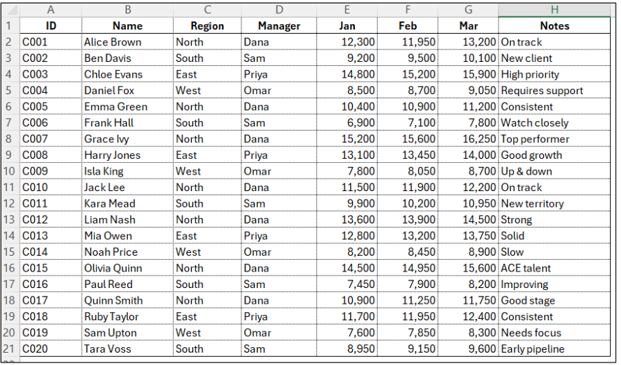
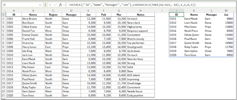
If we wanted to return:
- Columns 1, 2, 4, 5
- Last 10 rows
- Stack a custom header on top
Formula
=VSTACK({“ID”,”Name”,”Manager”,”Jan”},CHOOSECOLS(TAKE(A1:H21,-10),1,2,4,5))
Tips and Best Practices
1. Use TAKE before DROP for clarity
TAKE(…,5) is easier to understand than DROP(…,-5).
2. Use VSTACK for monthly/weekly data
Great for building master tables from data within monthly sheets.
3. Use CHOOSECOLS to simplify Power Query-style reshaping
You can create “views” of your data without ever touching the original table, keeping the data intact.
4. Dynamic arrays refresh automatically
Everything updates when source data changes – no manual copy/paste.
Conclusion
Each of these formulas is simple on its own, but the real power comes when you combine them. You can now reshape, extract, and consolidate data using a single formula, where previously you might have built a Pivot Table or made manual edits. That means less time wasted and far fewer human errors.
Mastering these functions dramatically reduces formula complexity and creates cleaner, more robust models, especially when paired with other dynamic tools like SORT, FILTER, and UNIQUE.