Eliminate the need for data cleansing by using Excel’s data validation tool, explains Traci Williams
On most spreadsheets, it won’t take us long to find a typo or a mismatch with abbreviations. Let’s face it, these mistakes are easily made, especially as we’re all so busy these days.
However, this means that before we can use the data in a spreadsheet for useful summaries, we’ll need to cleanse the data to make it consistent.
Wouldn’t it be great if we could make sure the data is right when it’s entered so we don’t have to go through the manual job of data cleansing!?
Excel has the perfect tool for this called Data Validation.
Data Validation
This tool can be used to ‘force’ the user to enter correct data. It’s super simple to use, and highly effective.
I use it all the time to prevent myself from making typos and entering data in an incorrect format.
I always recommend selecting the cells to apply the Data Validation to first; then go to the Data Ribbon and select Data Validation (top half of button):

The Data Validation screen appears as follows:
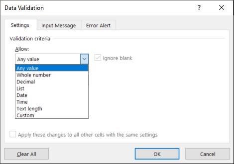
There are 3 tabs available. The first one is ‘Settings’ and is where we define the Data Validation criteria.
Settings
Every cell in an Excel spreadsheet defaults to ‘Allow any value’ (as can be seen in the above image). This allows us to enter anything we like into any cell until we start applying Data Validation.
There is a pick list in that box with eight different options to choose from, as follows:
- Any value: This is the default selection and allows the user to enter anything
- Whole number: The user can ONLY enter a whole number
- Decimal: The user can enter either decimals or whole numbers
- List: The user can select from a list (pick list / drop down list)
- Date: The user can ONLY enter a date using the format: dd/mm/yy
- Time: The user can ONLY enter a time using the format: hh:mm
- Text length: The user can only enter a specific number (or range) of characters
- Custom: Formulas and specific criteria can be entered using this option
For most of the above options, the user can also further restrict the data entry to a specific range of numbers or dates as required.
I’ll explain a few of these options:
List
Let’s say we want to restrict the data entry so that users can only enter:
- Yes
- No
- Maybe
We need to select List from the ‘Allow’ box:
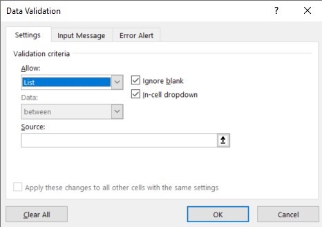
In the ‘Source’ box, we can just type in the options we want to allow, separating each one with a comma (a space can be used too, to make it easier to view):
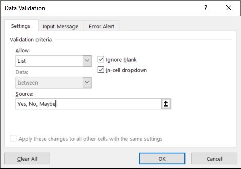
Then click ‘OK’ to return to the spreadsheet.
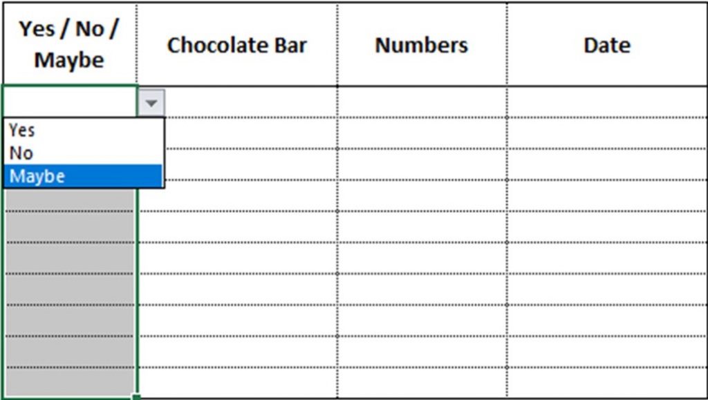
Each of the cells that was highlighted at the beginning will now contain an arrow to the right of the cell. Click on the arrow and the list items will appear in the same order in which they were entered.
The user can now select from the list to populate the cell with that value, saving having to type anything manually (increasing speed) and removing the risk of a typo or an incorrect abbreviation (increasing accuracy).
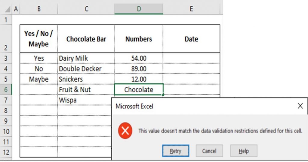
The user can still manually type into the cell, but the value must match an item from the list. If it doesn’t match, the user will see this message:
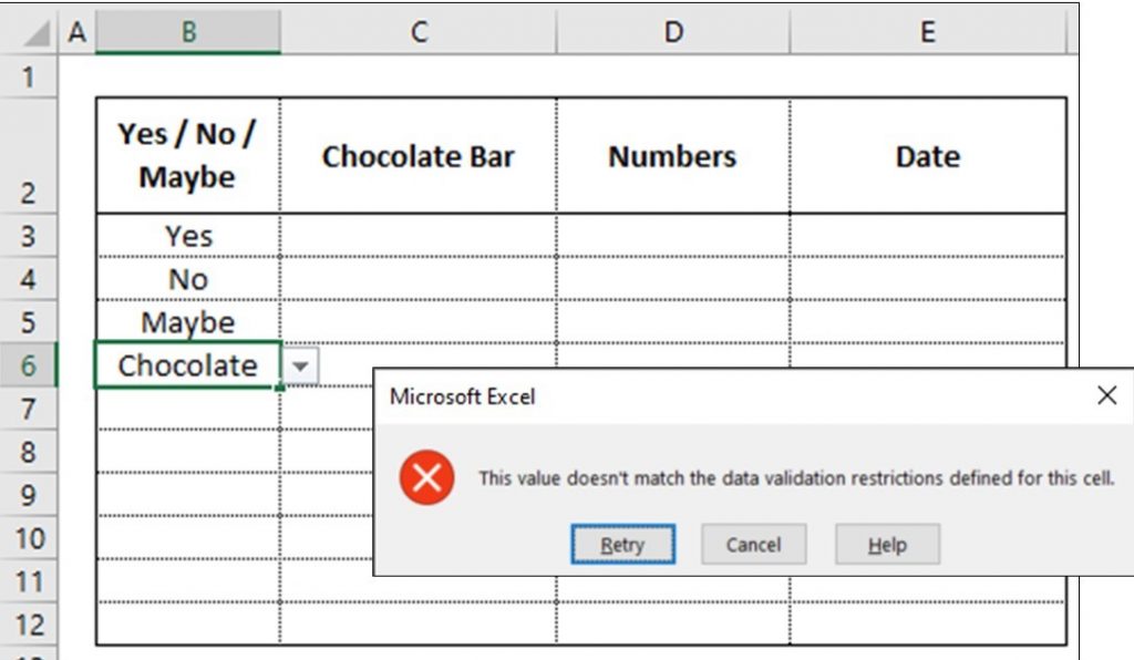
This error is saying that ‘Chocolate’ does not appear on the Data Validation List, and therefore it cannot be entered into this cell. The user has the option to ‘Retry’ in case they have made a typo, but ONLY values that appear on the list will be accepted.
Note: When the list is manually typed into the ‘Source’ box, as in the above example, the text also becomes case sensitive.
List (external source)
If we have a longer list of items to select from that change on a regular basis, it might not be very easy to type them into the Source box (as above), so the Data Validation can be linked to a range of cells instead.
Note: When the list is linked to an external source, it will NOT be case sensitive.
In the example below, column G includes a list of chocolate bars that I would like the user to select from within a pick list in column C:
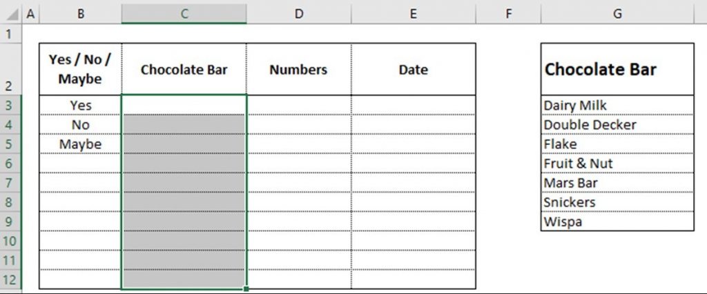
After highlighting the cells in column C, go to the ‘Data’ ribbon and select ‘Data Validation.’
Select List from the ‘Allow’ box, place the cursor in the ‘Source’ box, then navigate to the cells on the spreadsheet that form the list:
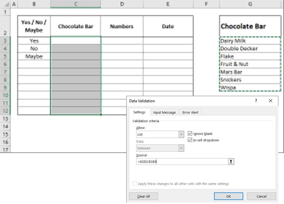
The selected range will appear in the Source box. Then press OK.
Each of the cells that was highlighted at the beginning will now contain an arrow to the right of the cell. Click on the arrow and the list items will appear in the same order in which they appear in the source list.
The user can now select from the list to populate the cell with that value:
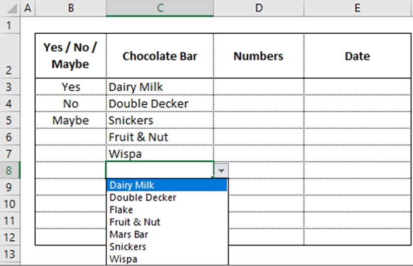
Of course, the list can also be edited, or sorted, in column G, and this will automatically update the pick list in column C.
Numbers
If we want to restrict column D so we can only enter numbers, we need to highlight the cells, then go to the ‘Data’ ribbon and select ‘Data Validation.’
Select Whole Number (or Decimal, as required) from the ‘Allow’ box:
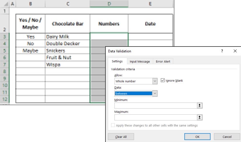
In the ‘Data’ box are all the usual options for numbers (i.e., between, greater than, less than, etc.), and then minimum and maximum values can be entered into the boxes below.
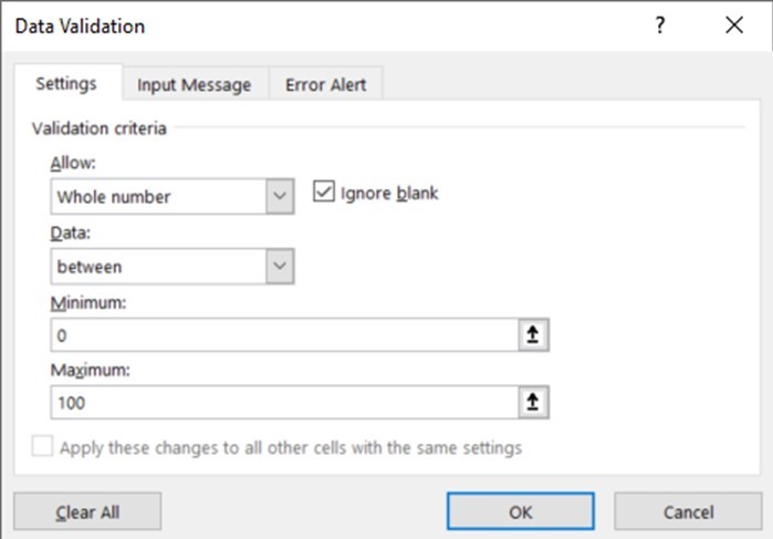
Then click OK.
Each of the cells in column D will not appear any differently, but you will be unable to enter anything except a number between 0 and 100. This means the user can only enter correct information (in the right format) into these cells.
If an incorrect value is entered, this error message will appear:

This error is saying that ‘Chocolate’ is NOT a value between 0 and 100 and therefore cannot be entered into this cell.
Date
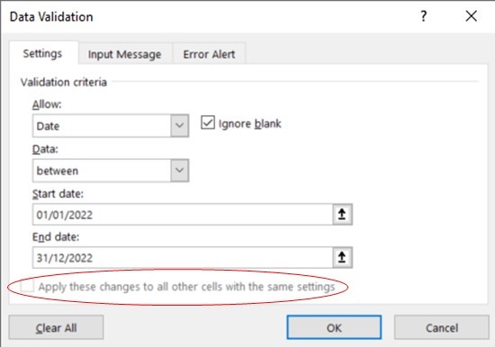
If we want to restrict column E so we can only enter dates from 2022, we need to highlight the cells, then go to the ‘Data’ ribbon and select ‘Data Validation.’
Select Date from the ‘Allow’ box:
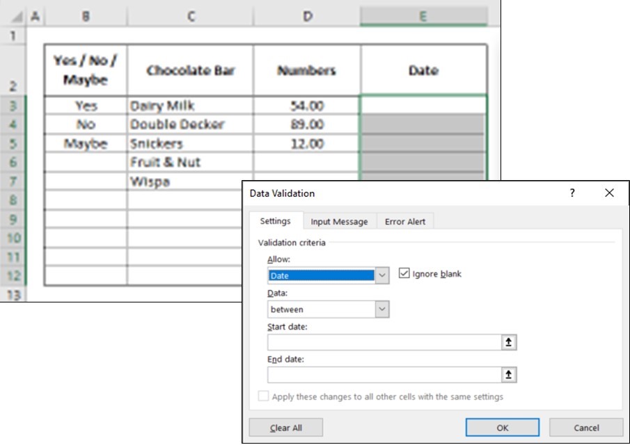
In the ‘Data’ box are all the usual options for dates (i.e., between, greater than, less than, etc.), and then start and finish dates can be entered into the boxes below.
Then click OK.
Each of the cells in column E will not appear any differently, but you will be unable to enter anything except a date within the year 2022 (formatted as dd/mm/yy). This means the user can only enter correct information (in the right format) into these cells.
If an incorrect value is entered, the user will see an error message like those for the other data types.
Note: I often include Data Validation for dates, even when I don’t mind what date is entered (using start date 01/01/1900 and finish date 31/12/3000), purely as this forces the user to use the correct date format (dd/mm/yy).
One last thing to note on the Settings tab: on the bottom left of the screen, there is a tick box to ‘Apply these changes to all other cells with the same settings’:
On first application of Data Validation, I recommend selecting all the relevant cells first, but if you want to amend an existing rule, you can simply select one of the cells and place a tick in this box, and it will automatically select all the cells with the same rule.
There are two further tabs in the Data Validation screen:
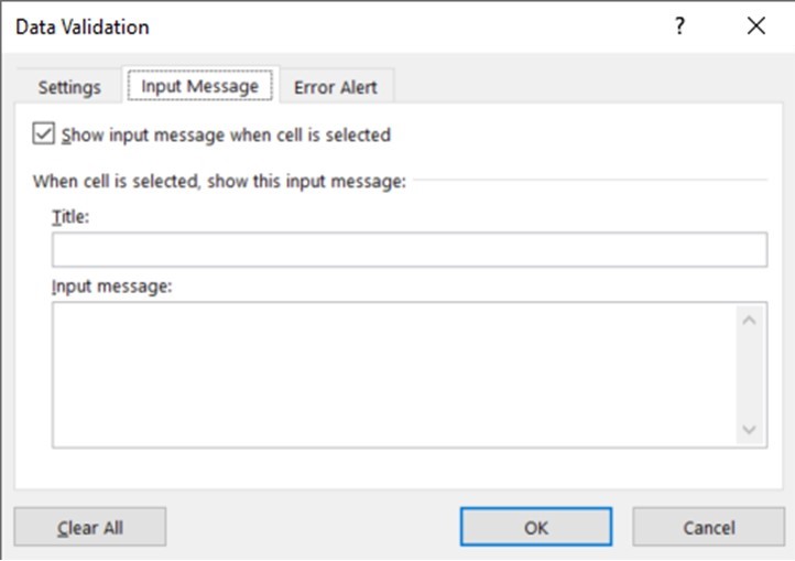
Input Message
In this tab we can enter a title and an input message to appear when the cells are selected. This is to give the user more information as to what they need to do when they select the cells:
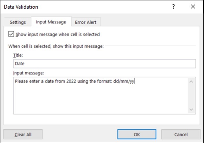
Click OK to return to the spreadsheet.
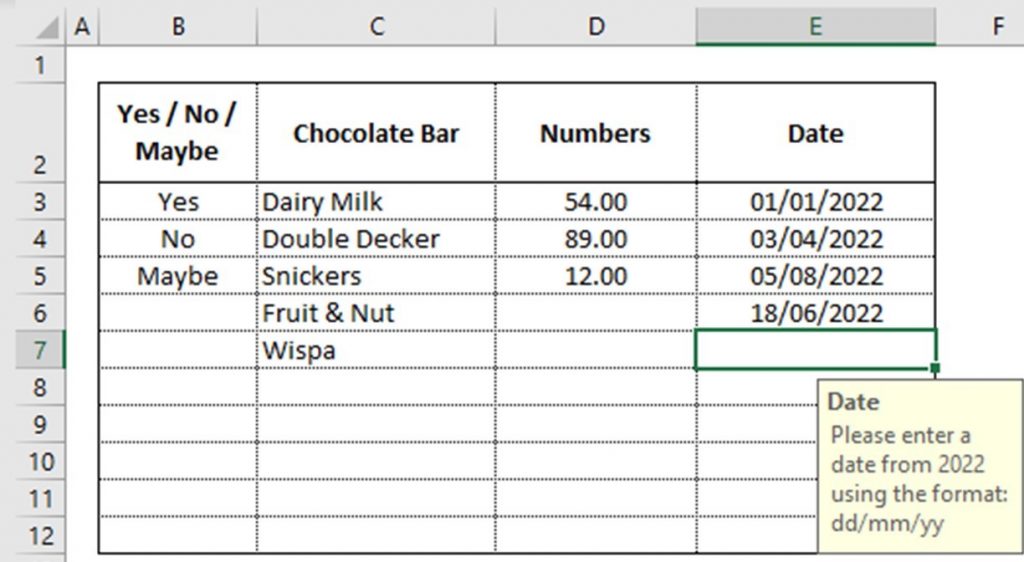
As each of the cells in column E is selected, a yellow pop-up box containing the message will appear to give the user more information:
Error Alert
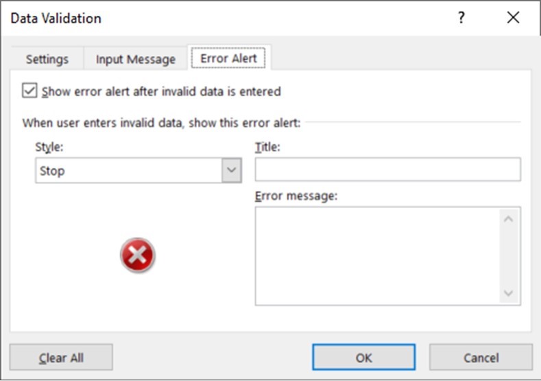
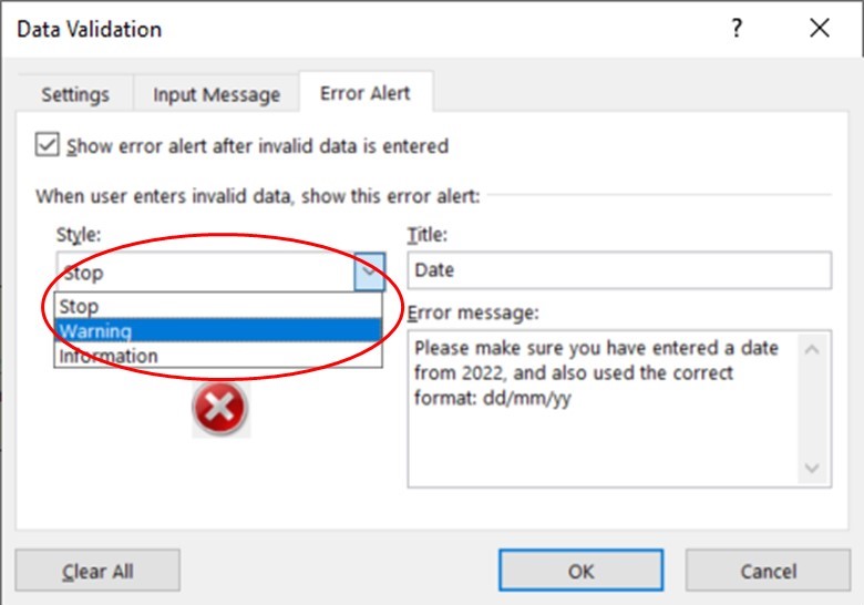
In this tab we can enter a title and an error message that will appear when the user enters invalid data. This will replace the somewhat unhelpful message that currently appears with something that can be tailored to help the user resolve the issue and complete the task:
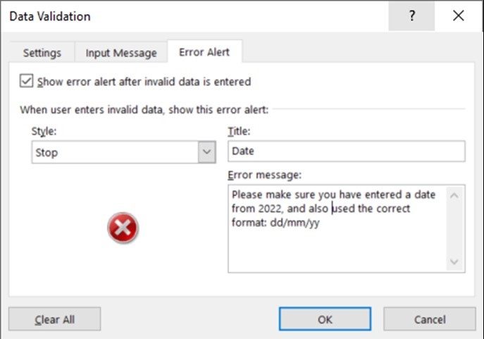
Click OK to return to the spreadsheet.
Now, when an invalid entry is made, the user will see this error message:
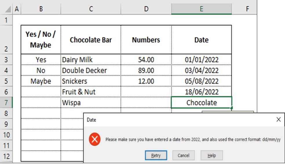
Also note that each of the error messages we’ve seen so far includes the cross in the red circle, and the user is unable to enter any data that does not meet the criteria. This is the due to the Data Validation style being ‘Stop,’ which is the default option.
There are two further options we can select:
Warning
This displays an exclamation mark in a yellow triangle and gives the user the option to accept the invalid data anyway:

The user can select ‘Yes’ to accept the invalid data, but this is a one off, and this message will appear every time incorrect data is entered.
If the user selects ‘No,’ they will have the option to amend the entry (similar to ‘Retry’ on the Stop style).
Information
This displays an ‘i’ in a blue circle and gives the user the option to accept the invalid data anyway:

The user can select ‘OK’ to accept the invalid data, but this is a one off, and this message will appear every time incorrect data is entered.
Conclusion
There are lots of ways that Data Validation can be used, and I genuinely use it in every spreadsheet, if only to protect myself from the dreaded typos!


