
Traci Williams shares her answers to the most common Excel questions she is asked
Excel Ace is celebrating its 15th year in business, which is just ACE and makes me very happy and grateful.
However, it has also made me reflect on how Excel has changed and developed over the years, and also on some of the questions I have been asked time and time again (and still am). I wanted to share 10 of the most common questions and answers, as I’m certain they may come in handy for you.
Some of these questions never get asked, as people tend to find a workaround, but then it feels as if Excel has a mind of its own and is not very easy to use.
Hopefully, these answers help you to understand just why Excel does some of the things it does…and that it’s ALWAYS trying to help.
1. Why Does Excel Drop the 0 on Phone Numbers?
When you type a phone number (or any number) into Excel, you’ll notice that after pressing ‘Enter’, the leading zero is removed:

Excel recognises data as being one of the following data types:
- Number
- Text
- Date
In the instance above, Excel has recognised that the data is a number, so it has formatted the cell as such. Excel deems that any leading zeros are irrelevant to a ‘number’ (which, of course, logically they are!), and therefore removes them.
There are a couple of ways to overcome this:
- Enter an apostrophe ( ‘ ) before the number. This includes a character AND a number, tricking Excel into not recognising the number and forcing Excel to format the cell as text and leave the 0 in.
- You could also include spaces in between the numbers, as this works in the same way as above but also makes the number easier to read and ensures there are enough digits.
- You could format the cell as ‘text’ BEFORE you enter the number…this way Excel won’t have to guess and will do as you’ve asked.
2. Autofill: Sometimes It Copies, and Sometimes It Fills Consecutively; How Can I Make It Do What I Want?
Autofill is when you drag a cell down (or up, left or right too) with your mouse, from the bottom right corner, and the data is copied.
This will usually appear similar to this:
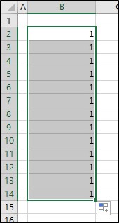
In this instance the data has been ‘copied’, so all cells now contain the same value.
Notice to the bottom right of the fill range, there is a little icon, and this represents your ‘Autofill Options’.
**I am always shocked by how many people have never clicked on this icon and don’t know about its ‘superpowers’.**
These options are as follows (left-click on the icon):
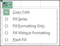
You now have control over which option you choose.
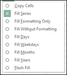
The Autofill Options vary slightly depending on the data in your original cell: the above options are for numbers.
The options for text will be the same, but exclude ‘Fill Series’, as Excel wouldn’t usually know what other text to include.
The options for dates are quite impressive:
3. Dates Are Not Appearing Correctly; They Look Like Numbers
In Excel, dates are treated as numbers, but in order for Excel to perform calculations with them, each date is given a ‘serial number’.
The very first date in Excel is 01/01/1900. That was assigned the serial number of 1, and those serial numbers increase sequentially.
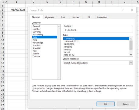
In the example below, the date is 01/02/2023, and the serial number is 44958.
The only reason the serial number is being displayed (and not the date) is due to the formatting of the cell being ‘General’, as you can see here:

If we changed the format of that cell to ‘Date’, it would appear as follows:
4. How Can I Highlight My Data Quickly?
There are a few ways to do this, and I am always keen to use these options, as it saves the mouse running off as you scroll down.
Ctrl + A: Position the cursor anywhere within the range you want to highlight, then press Ctrl + A and ALL adjoining cells will be selected.
Ctrl + Shift + End: Position the cursor at the top left of the data you want to highlight, then press Ctrl + Shift + End and ALL used rows and columns below the starting cell will be highlighted.
There are other combinations of Ctrl / Shift / End / Arrow keys that will give you more control, but the options above are the quickest.
5. How Can I Get My Sheet to Print on One Page?
You may remember the old ‘Page Setup’ menu to select your print options:
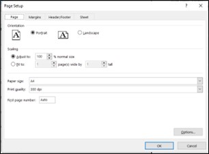
On this screen, it was a fine art to carefully select the number of pages ‘wide’ by pages ‘tall’ to get the printout on one page. And that was if you knew where it was.
Thankfully, in 2010, Microsoft amended the Print Preview screen, so we no longer need to use the ‘Page Setup’ menu (but it is still there if you want it or need to use some of the options from it).
This now looks as follows:
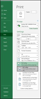
The bottom option defaults to ‘No Scaling’; simply left-click on it to view the other options. They are far easier to understand and clearly state ‘Fit Sheet on One Page’ or ‘Fit ALL Rows or Columns on One Page’.
6. The Filter Does Not Include ALL of My Data
When the Autofilter is first applied, if you have selected the entire range first, then it will be applied to that range. If rows or columns are inserted (or deleted) into that range, then the filter range will automatically adjust.
If the Autofilter is applied by selecting the header row (and NOT the entire range), then the range will be applied to all of the rows between the header and the first blank row. If your data does have blank rows, then you will certainly need to highlight the entire range (as above) before applying the Autofilter.
If data is added below the range and in an adjoining row, then the filter range will automatically adjust. However, if there is a blank row between the current range and any new data, then the filter will not include it in the range.
Any issues with the filter are always easily remedied by simply removing the filter, selecting the entire range, and reapplying the filter.
7. Vlookup Is Not Working
Excel is so logical that if it fails to return a valid answer to a formula, there will be a valid reason to explain it.
With Vlookup formula, if we assume the formula has been entered correctly, there are a couple of typical reasons for Vlookup formulas not to work:
Formatting
If the data is in two different formats (e.g., number & text), then it will be impossible for Excel to find a match for these. This can be tricky to spot, but here is an example:
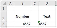
Although the cells both contain an identical number, cell B3 is formatted as a number (notice the value is aligned to the right) and cell D3 is formatted as text (notice the value is aligned to the left).
If we formatted both of these in the same way, Excel would be able to match the numbers and return a valid answer for the Vlookup.
Spaces
This can be the most frustrating and difficult issue to spot, as it is almost impossible. If text contains spaces at the end of the text, Excel recognises the space as another character, and again will not be able to match the text. The difficulty is that the spaces are invisible, so very tricky to spot!
Quick tip to identify spaces at the end (or in the middle) of text is to underline the cell, as this will highlight ALL characters, including the space, so you can see them:
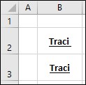
To resolve the issue with spaces, the obvious answer would be to remove the spaces, but if there were LOTS of cells with spaces, this could be very time-consuming.
I’d recommend using a TRIM formula within the Vlookup formula, as this will trim any irrelevant spaces within the text (before it is used in the Vlookup formula):
Original Formula: =VLOOKUP(B2,K2:K10,2,FALSE)
Formula with TRIM: =VLOOKUP(TRIM(B2),K2:K10,2,FALSE)
8. Red / Green (and Purple) Triangles Appear in Cells
These can appear as follows:

Red triangles
These appear in the top right corner of a cell. They were called ‘Comments’ (a long time ago), but now they’re known as ‘Notes’.
To enter a note, right-click on a cell and select ‘New Note’; you can then enter any text as required.
Notes will appear as a pop-up as you select the cell, or you can make them always visible (right-click on a cell with a note to see the options).
Green triangles
These appear in the top left corner of a cell and are ‘Warnings’; they will appear as Excel notices anything it thinks you might want to know.
If you select the cell with a warning, you’ll see an icon with an exclamation mark appear on the left. Left-click on this icon to see the warning and the various suggested solutions. The warnings will not cause any issues but are useful to have a look at in case you’ve missed something.
Purple triangles
These are fairly new (since 2019) and also appear in the top right corner of a cell. They represent ‘Comments’, which are date and time stamped and also include the User ID. These can be entire conversations, where you can tag other users and even reply to their comments.
9. How Can I Copy a Whole Sheet?
The usual way would be to right-click on the sheet name and select ‘Move or Copy’, and this menu will appear:
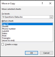
Here you can select the file to move or copy to, the position within the existing sheets, and whether to copy the sheet or move it.
However, there is a far simpler way, and that is to select the sheet, hold down the Ctrl key, and drag the sheet with the mouse to the position you want it in. The new sheet will be renamed initially with (2) after the name, and you can amend it as required.
10. Why Do You LOVE Excel So Much?
I have been using Excel for more than half my life, and I love the logic of it and how there is always a solution to be found. There is no greater feeling than cracking that formula or VBA code that will help make someone’s life easier.
I love working with people who don’t like Excel (or worse, are fearful of it) and helping to show them the simplicity of what they need to know, and seeing the look of relief on their faces as their fears disappear.
Excel also keeps changing and developing, so there is always so much for me to keep learning…and falling in love with, of course!


