
Traci Williams introduces us to two brand new and shiny formulas in Excel!
These two formulas were first released in BETA back in 2023 but have only been rolled out to ‘Current Channels’ in the last few months.
Say hello to GROUPBY and PIVOTBY:
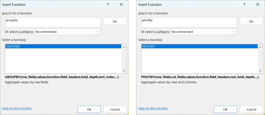
As you can see, the Groupby formula will consolidate values into rows, and the Pivotby formula will provide both rows and columns, just like a Pivot Table.
GROUPBY
We can use the Groupby formula with this data (columns A:F) to summarise Total Quantity by Sales Rep as follows (see formula in cell H1):
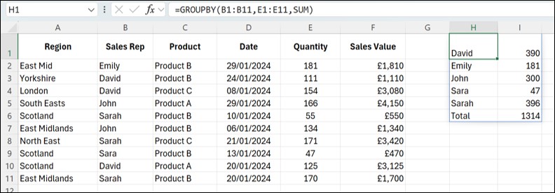
To enter this formula, you can either use the wizard or just use the syntax that appears as you start typing the formula, not the cell (both have pros and cons).
Using the wizard, search for the Groupby formula:
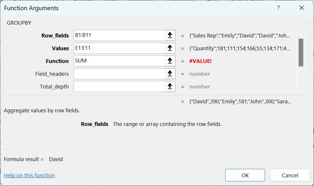
Any descriptions in BOLD are mandatory, where those in regular text are optional.
The fields are as follows:
Row_fields: The range to summarise (e.g., Sales Rep)
Values : The range to aggregate (e.g., Quantity)
Function: This is the calculation to apply (17+ available)
(if left blank, no headers will be included)
Field_headers: A number between 0-3 to signify use of headers
Total_depth: A number between 0-2 to signify use of totals
(if left blank, a grand total will be included)
Using the wizard is not terribly helpful in terms of the options available for the ‘Function,’ ‘Field_headers’, and ‘Total_depth’. You can find pick lists for these by accessing the syntax on the face of the spreadsheet instead.
Press F2 on the cell containing the formula to open the cell for editing, then click on any part of the formula, and the syntax will appear beneath the cell, highlighting in BOLD the area that has currently been selected.

If you remove the word ‘Sum’ from the above formula, you will see the list of available calculations:
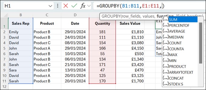
There are 17 on this list, but the last one is ‘LAMBDA’, which can be used to create your own unique formulas.
If you enter a comma after the ‘Function’ selection, you will see a pick list for the ‘Field_headers’ (i.e., headers for columns) as follows:

If you enter a comma after the ‘Field_headers’ selection, you will see a pick list for the ‘Total_depth’ (i.e., totals for columns) as follows:

From the above syntax, you can recognise the first five fields, as they replicate the fields we saw in the wizard; however, you can also see here that there are a further three fields available (also shown inside square brackets ( [ ] ), making them ‘optional’ choices). They are:
Sort_order: A number to determine how the output should be sorted.
The number represents the column number; a positive number
represents ascending order while a negative number represents descending order.
Filter_array: Filter the result by a specified criterion
Field_relationship: Either Hierarchy (0) or Table (1)
In the below example, I have amended the Groupby formula to include both
Quantity AND Sales Value (B1:C11),
by Sales Rep AND Product (E1:F11),
including Headers (3), Subtotals, and Grand Totals at the top (-2),
sorted in Descending Order of Sales Value (-4):
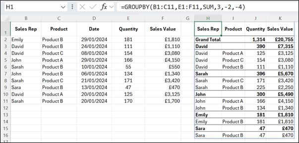
This is quite an impressive output from just ONE (relatively small) formula!
NOTE: I’ve used Conditional Formatting in the above, to include BOLD text and borders on the rows containing totals.
PIVOTBY
This formula is fairly similar to Groupby, but gives an added dimension of being able to include columns as well as rows to create a table or matrix style output:

As above, we can use either the wizard or the syntax to enter this formula.
This is how the wizard appears:
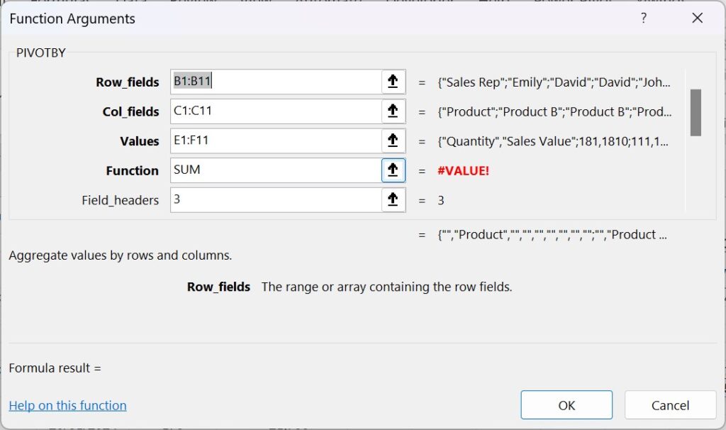
The fields are as follows:
Row_fields: The range to summarise by row (e.g., Sales Rep)
Col_fields: The range to summarise by column (e.g., Product)
Values : The range to aggregate (e.g., Quantity / Sales Value)
Function: This is the calculation to apply (17+ available)
Field_headers: A number between 0-3 to signify use of headers
(if left blank, no headers will be included)
As with the Groupby formula, the wizard does not provide the pick lists, but these are available from the syntax on the face of the spreadsheet instead.
The output of this formula appears very similar to a Pivot Table.
One other major advantage of using Pivotby is that, unlike a Pivot Table, we can use this formula to summarise text.
In this example, the regions covered by each sales rep have been summarised using the Pivotby formula:
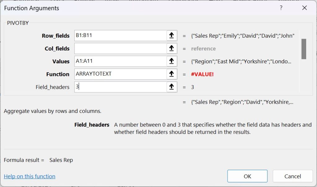
The wizard for this output looks like this:

Row_fields: Represents the Sales Rep column
Col_fields: This has been left blank
Values: Includes the Region column
Function: Does not represent a mathematical calculation, but uses the
‘ARRAYTOTEXT’ function, which separates each word with a comma and a space
Field_headers: Yes & Show (3)
Comparison to Alternatives
Of course, before these formulas were invented, we would have had to use multiple formulas to achieve such results, such as:
Unique & Sumif (instead of Groupby).
Before the invention of the ‘Unique’ formula, we would have needed to manually list the items or generate the list using a Pivot Table.
Pivot Table (instead of Pivotby)
Concatenate (instead of Pivotby)
This required knowledge and skill of these formulas and techniques, and usually also required lots of manual amending and reconciliation if (or when) the data changed. But with these new formulas, we can eliminate a lot of that manual work and reduce the risk of errors.
Pros and Cons
It’s always difficult to adapt to change, and looking at the number of fields for each formula, they do look like they can be quite tricky to master; however, here are some pros and cons to mastering them:
Pros
- Automatic recalculation, don’t need to manually refresh a Pivot Table (or rely on VBA)
- One formula as opposed to requiring multiple formulas or building and maintaining a whole Pivot Table
- Dynamically updated as data changes, don’t need to manually extend range or formulas
- Pivotby can use text, not just numbers…this is new and very exciting!
- Additional calculations available that do not exist in Pivot Tables
- Easier to ‘Sort’ results
Cons
- You cannot link Slicers or Timelines to Pivotby formulas
- You cannot link Pivot Charts to Pivotby formulas
- Not as easy to apply formatting as it is to Pivot Tables
- Means learning new techniques and skills (also a Pro!)
Conclusion
Like with everything in Excel, there are always different ways to do everything, and these formulas represent exciting new opportunities for users to upskill themselves, increasing productivity and efficiency.
I will absolutely be looking out for every opportunity to include these new formulas in my spreadsheets going forward.
Here is a link to a video demo of these formulas too: https://youtu.be/gi_8AtAvG20


