Traci Williams explains how to protect formulas from being overwritten
Have you ever been filling in a spreadsheet, and realised you’ve accidentally typed over your formulas? Or you’ve put your blood, sweat and tears into designing THE perfect spreadsheet, only for someone else to overwrite your beautiful formatting or formulas?
It can be very frustrating, but I have good news: there is a way to ‘protect’ your spreadsheets from this very thing.
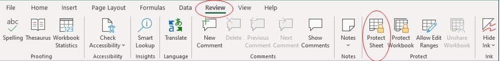
The function you need is called ‘Protect Sheet’ and is in the ‘Review’ ribbon:
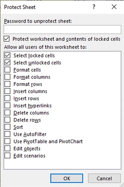
When you press this button, this screen will appear:

This includes a tick in the box (at the top) for:
‘Protect worksheet and contents of locked cells’
This means that when this sheet is protected, the user will be unable to edit any ‘LOCKED’ cells on this sheet.
Locked / Unlocked Cells
By default, EVERY cell in Excel is locked; therefore, when we protect the sheet, we will be unable to edit any cells at all – unless, of course, we ‘unlock’ them first.
In the example below, I have colour coded the cells as follows:
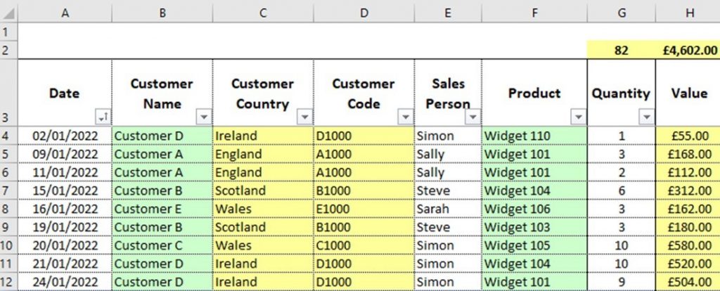
Green – Pick List (Data Validation)
White – Manual Entry (no restriction)
Yellow – Formula (DO NOT EDIT)
I would like to still be able to edit the green and white cells, even when the sheet is protected, and just have the yellow cells locked from editing.
To do this, I would need to ‘UNLOCK’ the green and white cells first:
- Select all cells to unlock
- Right-click mouse
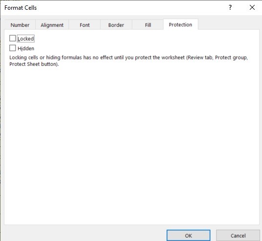
- Select ‘Format cells’
- On the ‘Protection’ tab, untick the ‘Locked’ box
- Click OK
Once the sheet is protected, you’ll notice you are now able to edit the green and white cells, and only the yellow cells (and those outside of the range) will be protected and uneditable.
Top tip
I always colour code cells to give me a visual guide as to how to complete them as well as to make them look neat and interesting. It also makes it easier to give directions to others when you can direct them by colour, instead of cell/row or column references.
Hidden
In the ‘Protection’ tab above, there is a second box called ‘Hidden.’
I would usually tick this box for any cells that contain formulas (usually coloured yellow, and also locked).
This means that when the sheet is protected, the user is unable to see any formulas. The formulas still work and recalculate, but the user is unable to view them.
It also means that if the user ‘copies’ and ‘pastes’ these cells, only the value is pasted, and not the formula.
There are a couple of reasons why this is useful:
- People often feel uncomfortable/scared when they see formulas (especially the big ones), even if they don’t need to edit them. If they don’t need to see them, it makes sense to keep them hidden.
- It prevents people from copying your clever formulas and passing them off as their own work.
- It acts as a deterrent to stop someone from copying a protected sheet, as they will need to replace the formulas or make the calculations manually.
Password
Protection can be added with or without a password.
Passwords ARE case sensitive, can be any length and can contain letters, numbers or characters. Once you enter the password and press OK, you will be prompted to re-enter the password as follows:
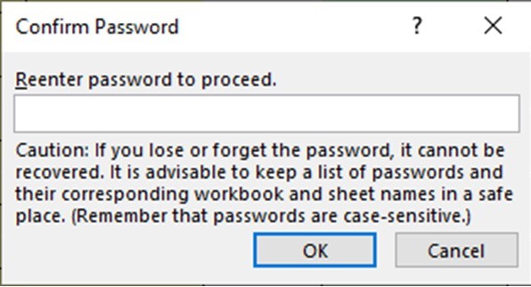
Please note the warning in the box above: passwords cannot be recovered. There is no official solution offered by Microsoft to retrieve forgotten passwords, so please ensure you use something memorable.
I usually only use a password if I am sending a file externally. If I am adding the protection for my own benefit, I usually leave the password off (just to make it quicker to remove if I need to).
Switching Protection On and Off
From this screen (‘Review’ ribbon, ‘Protect Sheet’), if you don’t want a password, simply click OK, and the sheet will be protected:
Or if you do want to use a password, enter it into the box above, then re-enter on the above screen and press OK.
When the sheet is protected, you may notice some of the icons on some of the ribbons are greyed out (e.g., the spell check icon below), and also the name of the button in the ‘Review’ ribbon has changed to ‘Unprotect Sheet’:
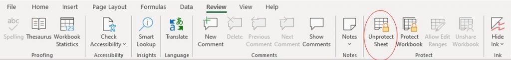
When you want to remove the protection, simply click on the ‘Unprotect Sheet’ button above.
If there is NO password, the protection will just be removed.
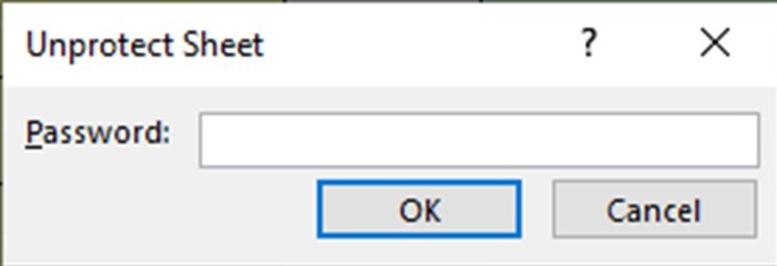
If there IS a password, you will be prompted to enter the password:
If an incorrect password is entered, you will see this message:
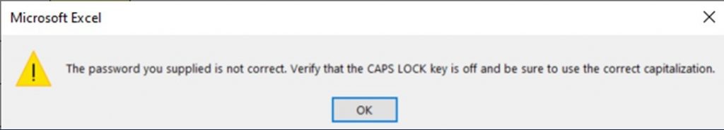
You have unlimited attempts to enter this password correctly, without being locked out.
Once the correct password is entered, the protection will be removed, and Excel will forget the password used, so you can use a different password next time (if you choose).
Allow Users to Use Functions
When a sheet is protected, the default functions that can be used are only the top two:
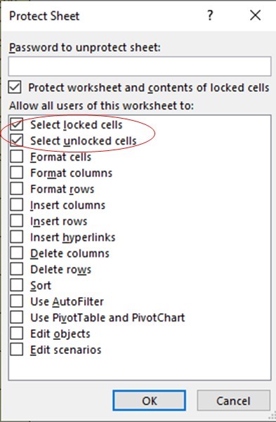
They literally mean that users can select ALL cells, whether locked or unlocked.
If the ‘Select locked cells’ box was unticked, users would be unable to select locked cells, which negates the need to hide the formulas.
You can manually select any of the other options that you would like the user to be able to use whilst the sheet is protected. Most of them are self-explanatory, but the ones I find most helpful (and use regularly) are:
Format columns: This means users can amend column widths
Sort: This is a bug in Excel; even when ticked, the user is still unable to use the Sort function
Use AutoFilter: Filter is temporary anyway, so can’t do any harm
Use PivotTable & PivotChart: This enables users to edit filters / slicers & timelines
The protection is applied to the currently selected sheet ONLY.